Exhibit 99.(8)
INTRODUCTION
The Economic and Financial Document 2019, the first of the new Government, examines the results
achieved in ten intense months of activity and traces the budgetary and reform policy strategy for the next three years. The Government has fully realised the initial economic and social reform programme described in early autumn in the Update of the
EFD 2018. This happened in an international and European economic context that has become increasingly difficult and in the presence of periods of tension in the government bond market. The Government has tackled the situation by modifying its
initial budgetary plan in order to reach an agreement with the European Commission at the end of last year, but that has not prevented the realisation of its reform and social inclusion goals.
Albeit in a deeply changed and more complex short-term economic context, with this document the
Government confirms the fundamental objectives of its action: gradually reducing the growth gap vis-à-vis the European average that has characterised the Italian economy especially in the last decade, while at the same time lowering the debt-to-GDP
ratio. To this end, the Government’s strategy reaffirms the role of public investment as a crucial factor for growth, innovation, social development and increased competitiveness of the production system; tax reform in a gradual transition towards a
flat tax system as an important component of a more balanced growth model; support to companies engaged in technological innovation and the simultaneous strengthening of the social protection and inclusion system.
The difficult economic situation that we face today is characterised by a decline in manufacturing
activity that has particularly affected both Germany and Italy due to their production specialisation and their high export orientation. International relations have changed greatly in the last two years and the evolution of world trade has reflected
this to a growing extent. This is compounded by the slowdown of some major emerging economies, the depreciation of the respective exchange rates, continuing uncertainty surrounding Brexit and the regulatory and technological changes that have
affected the automotive industry. These trends have resulted in a marked slowdown of European growth, which is accompanied by persistent conditions of low inflation. These conditions are more favourable for the countries most affected by the crisis
at the beginning of the decade, such as Italy.
In this context, our country’s performance shows that employment and the value added of services
have been maintained, but this has not been sufficient to
|
ECONOMIC AND FINANCIAL DOCUMENT 2019
|
ensure an adequate rate of growth in Gross Domestic Product. Year 2018 ended with an increase in real GDP of 0.9 percent,
affected by the unfavourable dynamics of the second half of the year that also determined a slightly negative carryover effect on 2019. Because of changes in the internal and external conditions, the growth projection for this year has been revised
downwards from 1 percent in the year-end forecast to 0.1 percent in the present document.
Overcoming this phase of low nominal growth in our economy depends on the evolution of the
international economy and the effectiveness of growth-stimulating policies, both macroeconomic and for structural reform, which we are implementing.
There is also a need for a change at European level to move to a growth model that, without
prejudice to the competitiveness of the EU countries, is based more on the promotion of domestic demand. The extremely high trade surpluses of some European countries represent the macroeconomic imbalances that are the source of excessive exposure to
shocks external to the Union, especially in an historical time in which globally we are witnessing a possible change of approach with respect to international trade and multilateralism. Therefore, at European level the Government will promote a
reappraisal of the economic policy approach, from the budgetary rules to industrial, trade, investment and innovation policies.
The current phase of cyclical weakness of the economy makes it necessary to sustain economic
activity and in particular public and private investment, which, though recovering, stood at 18 percent of GDP in 2018, compared to levels above 20 percent in the years before the crisis.
The Government has put in place two packages of measures to support investment. The first, the
‘Growth’ Decree Law, focuses on measures to stimulate the accumulation of capital and investments. Among other measures super-depreciation is reintroduced, modified so as to favour small and medium-sized enterprises, the mini-IRES (corporate income
tax) is replaced with a reduction in the rates of direct taxes on income attributable to profits retained in the undertaking and the procedures to benefit from the patent box tax relief are simplified. The measures to support private investment are
accompanied by an increase in budgetary resources for investment by local and regional authorities. Resources that are added to the expected positive effects in terms of greater investment attributable to the measures to release surpluses introduced
with the Budget Law for 2019.
The second measure, the ‘Sblocca cantieri’ (‘Unlock sites’) Decree Law, aims to boost the resumption of the
construction sector, streamlining the existing legislation relating to the award of contracts, integrated contracts, subcontracting, rules on planning, public-private partnership and the procedures
|
IV
|
MINISTRY OF ECONOMY AND FINANCE
|
|
INTRODUCTION
|
for the approval of project variations. Investment in construction increased last year by 2.6 percent and the number of
building permits considerably increased. The improvement of the regulatory framework resulting from the legislative intervention, together with the Government’s commitment to increase resources for public investment and incentives for the building
renovation, including for earthquake protection, should therefore create the conditions for a true recovery of a sector that is still crucial for employment and the general trend of the economy.
These interventions have a neutral impact on public finances, testifying the Government’s attention
to budgetary discipline. In the year-end agreement with the European Commission, the Government had indicated a net borrowing forecast for 2019 of 2 percent of GDP. The Budget Law contains a clause, which in case of deviation from the net borrowing
target envisages a block on two billion of public expenditure. Based on new forecasts published in this document, this scenario now appears likely. The Government will therefore implement this expenditure reduction.
Because of activating the expenditure reduction laid down by the legislation in force (which does
not therefore constitute an ‘additional measure’), the deficit for this year is estimated at 2.4 percent of GDP. In structural terms, i.e. net of cyclical component and temporary measures, this result would give rise to a variation in the net
borrowing of only -0.1 percentage points. Taking into account the flexibility agreed with the Commission in relation to extraordinary expenditure to tackle hydrogeological risks and extraordinary interventions on infrastructure, as well as the
negative level of the output gap, the result for this year would fall within the limits of the Stability and Growth Pact (SGP).
For subsequent years, the Stability Programme traces a public finance path that gradually reduces
the deficit of the general government to 1.5 percent in 2022, with a reduction of 0.3 percentage points per year that determines an almost equivalent improvement in the structural balance. According to the new official projections, the structural
deficit would fall by 1.5 percent of GDP this year to 0.8 percent in 2022, in line with a gradual convergence toward the structural balanced position. The planned policy objectives are in line with the SGP while setting more contained improvements in
the structural balance in comparison to a literal interpretation of the rules, as imposed by the still difficult conditions in which our economy finds itself and the recent cyclical weakening.
The expected trend of inflation and the GDP deflator for the current year and the next three years remains marked by a
strong moderation, making it more difficult to attain a high nominal growth and a marked reduction of the public
|
MINISTRY OF ECONOMY AND FINANCE
|
V
|
|
ECONOMIC AND FINANCIAL DOCUMENT 2019
|
debt ratio. The new official forecasts indicate an increase in the debt-to-GDP ratio for 2019, which moderately
increased last year. For the next few years, the Stability Programme aims for a reduction of the debt-to-GDP ratio, which would be close to 129 percent in the final year of the forecast.
As regards the internal budgetary policy targets, the policy scenario presented here expects an
increase in public investment over the next three years, which would rise from 2.1 percent of GDP recorded in 2018 to 2.6 percent of GDP in 2022.
In line with the Government Contract, it is also intended to continue, in the draft
Budget Law for next year, the process of reform of income taxes (‘flat tax’) and general simplification of the tax system,
by alleviating the taxation of middle classes. This in compliance with the public finance targets defined in this document.
The profile outlined for the net borrowing, also in light of the costs necessary for the
refinancing of so-called unchanged policies (peace missions, public employment, investments), will require the identification of large incremental resources. The existing legislation on tax matters is now confirmed pending the definition of
alternative deficit-reducing measures and tax reform measures in the course of the next few months, in preparation of the 2020 Budget Law.
The GDP growth forecast in the policy scenario, although affected by budgetary constraints, is
higher than that of the scenario based on unchanged legislation except in the final year, amounting to 0.2 percent in 2019 and then increased to 0.8 percent in the three following years (compared to a scenario at unchanged legislation that reflects
real growth rates of 0.6 percent in 2020, 0.7 percent in 2021 and 0.9 percent in 2022). Looking at the most recent forecasts of international institutions, it is observed that, although in a context of slowdown, in 2020 our economy is expected to
reduce the growth gap compared with the average of the countries of the euro area and the major European economies (France and Germany).
In general it is appropriate to reiterate what has already been stated in the past, i.e. that the
official forecasts are and must be of a prudential nature, as they are aimed at building a reliable and shared public finance framework. The Government aims to achieve much more significant results in terms of economic growth within an approach
that pays attention to the dimension of fair and sustainable well-being.
Reforms are the best way to enhance the economy's growth potential. This year’s National Reform Programme, the first
presented by the new Government,
|
VI
|
MINISTRY OF ECONOMY AND FINANCE
|
|
INTRODUCTION
|
reflects the various measures and reforms already undertaken and sets forth the strategy for the next three years.
The Government has prioritised social inclusion, fighting poverty, helping the inactive
population find employment and improving education and training. The ‘Dignity’ decree aims to reduce job insecurity by discouraging the excessive use of fixed-term contracts and promoting the use of permanent contracts. Citizenship Income has the
dual purpose of fighting poverty and helping beneficiaries in terms of job seeking and training paths.
The revision of the pension system through the so-called ‘Quota 100’ intends to allow easier
access to the pension, also favouring generational turnover and the innovation and productivity of businesses and public administrations.
The theme of the work will continue to have a central place in the Government’s economic policy
action over the next few years with the aim of ensuring fairer working conditions for Italian citizens and adequate wages. The introduction of a minimum hourly wage for those sectors not covered by collective bargaining and the provision of fair
treatment for apprenticeships in free professions will be subject to evaluation. Measures will be also considered to reduce the tax wedge on labour and cut administrative costs, including through digitisation.
In addition to investment in physical infrastructure, economic development requires also a
large effort in the field of technological innovation and research. The Government will draw up National Strategies for Artificial Intelligence and for Blockchain. Significant resources will be invested in the diffusion of broadband and the
development of the 5G network. The measures of the ‘Impresa 4.0’ Plan and those to support innovation in small and medium enterprises were also refinanced.
The Government will re-launch Italy’s industrial policy, with the aim not only of revitalising
sectors that have been in crisis for some time, but also to give Italy a leading role in industries that are at the centre of the transition toward a sustainable development model. The passage to higher ecological standards represents a real
opportunity for growth for Italy, which must be pursued by incentivising the research, design and production of means of transport with low environmental impact in our country. The Government will strengthen its support for trialling and adopting
digital transformations and enabling technologies that offer solutions for more sustainable and circular production. Green finance can provide an important contribution to the growth of these activities and the Government will support their
development.
Administrative simplification actions will be part of a more general measure to accelerate growth that the
Government intends to launch in the coming months, which will involve the recognition, typing and reduction of permission
|
MINISTRY OF ECONOMY AND FINANCE
|
VII
|
|
ECONOMIC AND FINANCIAL DOCUMENT 2019
|
regimes, identifying the non-essential authorisation procedures and eliminating unnecessary administrative burdens.
The efficiency of justice represents a decisive factor for economic recovery and for renewing
citizens’ confidence in the law. In this context, interventions aimed at speeding up civil and criminal judicial proceedings have been implemented, such as the comprehensive reform of insolvency proceedings, in addition to the important
resources allocated to solve staff shortages of administrative staff and the judiciary.
In addition, Italy has been characterised for years by the decline in the birth
rates and low female participation in the labour market. The Government intends to continue the efforts to reduce tax burden and allocating more resources in favour of families, with particular regard to large ones and those with a family
member with disabilities. Future initiatives will focus primarily on reorganising the subsidies for birth rates and parenthood, promoting corporate welfare for relatives, improving the healthcare
system and the related infrastructure.
Finally, one of the main policy-scenario targets of the Government’s action is to support
school and university education and research through measures to finance their development, with particular attention to human capital and infrastructure.
In summary, the key objective of the Government’s programme is a return to a phase of
economic development marked by an improvement of social inclusion and quality of life, ensuring the reduction of poverty and guaranteeing access to training and employment, while acting also in the perspective of reversing the negative
demographic trend. Regarding competitiveness, the Italian economy will be strengthened by the improvement of the productive environment caused by the reduction in costs for businesses, both fiscal costs and more generally those inherent in the
bureaucratic system.
|
Giovanni Tria
|
|
|
Minister of Economy and Finance
|
|
VIII
|
MINISTRY OF ECONOMY AND FINANCE
|
CONTENTS
| I. |
OVERALL FRAMEWORK AND BUDGTARY POLICY OBJECTIVES
|
| I.1 |
Recent trends and prospects for the Italian economy
|
| I.2 |
Macroeconomic scenario and public finance trends
|
| I.3 |
Public finance policy scenario and official macroeconomic forecast
|
| II. |
MACROECONOMIC FRAMEWORK
|
| II.1 |
The international economy
|
| II.2 |
Italian Economy
|
| III. |
NET BORROWING AND PUBLIC DEBT
|
| III.1 |
Final data and forecasts at unchanged legislation
|
| III.2 |
Public finance: policy scenario
|
| III.3 |
Financial impact of the measures of the National Reform Programme
|
| III.4 |
Trend of debt-to-GDP ratio
|
| III.5 |
The debt rule and the other relevant factors
|
| IV. |
SENSITIVITY AND SUSTAINABILITY OF PUBLIC FINANCES
|
| IV.1 |
Short-term scenarios
|
| IV.2 |
Medium-term scenarios
|
| IV.3 |
Long-term scenarios
|
| V. |
QUALITY OF PUBLIC FINANCES
|
| V.1 |
Actions taken and trends for the future years
|
| VI |
INSTITUTIONAL ASPECTS OF PUBLIC FINANCES
|
| VI.1 |
Recent legislative developments on the reform of the State budget
|
| VI.2 |
Budgetary rules for local government
|
|
MINISTRY OF ECONOMY AND FINANCE
|
IX
|
|
ECONOMIC AND FINANCIAL DOCUMENT - SECT. I STABILITY PROGRAMME
|
INDEX OF TABLES
| Table I.1 |
Summary of macroeconomic framework based on unchanged legislation
|
| Table I.2 |
Summary of macroeconomic framework based on policy scenario
|
| Table I.3 |
Public finance indicators
|
| Table II.1 |
Macroeconomic scenario based on unchanged legislation
|
| Table II.2 |
Base assumptions
|
| Table II.3a |
Macroeconomic prospects
|
| Table II.3b |
Prices
|
| Table II.3c |
Labour market
|
| Table II.3d |
Sectoral accounts
|
| Table III.1 |
General government budgetary prospects
|
| Table III.2 |
Differences compared to the previous Stability Programme
|
| Table III.3 |
Cash balances of the state sector and the public sector
|
| Table III.4 |
Flexibility granted to Italy in the Stability Pact
|
| Table III.5 |
Cyclically adjusted public finance
|
| Table III.6 |
Expenditure to be excluded from the expenditure rule
|
| Table III.7 |
Scenario at unchanged policy
|
| Table III.8 |
Significant deviations
|
| Table III.9 |
Financial impact of the measures in the NRP grids
|
| Table III.10 |
Public debt determinants
|
| Table III.11 |
General government debt by subsector
|
| Table III.12 |
Compliance with the debt rule: forward looking criterion and cyclically adjusted debt
|
| Table IV.1 |
Heat map for the variables underlying the S0 indicator for 2018
|
| Table IV.2 |
Sensitivity to growth
|
| Table IV.3 |
Expenditure on pensions, healthcare, care for the elderly, education and unemployment benefits
|
| Table IV.4 |
Sustainability Indicators
|
| Table V.1 |
Cumulative effects of the latest measures implemented in 2018 on general government net borrowing
|
| Table V.2 |
Cumulative effects of the latest measures implemented in 2018 on general government net borrowing
|
| Table V.3 |
Cumulative effects of the latest measures implemented in 2018 on general government net borrowing by subsector
|
| Table V.4 |
Effects of Decree-Law No. 109/2018 on general government net borrowing
|
| Table V.5 |
Effects of Decree-Law No. 113/2018 on general government net borrowing
|
| Table V.6 |
Effects of Decree-Law No. 135/2018 on general government net borrowing
|
| Table V.7 |
Effects of the 2019-2021 public finance budget and initial measures in 2019
|
| Table V.8 |
Effects of the 2019-2021 public finance budget on general government net borrowing
|
| Table V.8-A |
Effects of Decree-Law No. 4/2019 on general government net borrowing
|
|
X
|
MINISTRY OF ECONOMY AND FINANCE
|
|
CONTENTS
|
| Table V.9 |
Effects of the 2019-2021 public finance budget and initial measures in 2019 on general government net borrowing by subsector
|
| Table V.10 |
Effects of the 2019-2021 public finance budget on general government net borrowing
|
| Table V.11 |
Effects of Decree-Law No. 4/2019 on general government net borrowing
|
INDEX OF FIGURES
| Figure I.1 |
Gross domestic product
|
| Figure I.2 |
Relative industrial production index, Germany vs Italy
|
| Figure II.1 |
Global composite PMI and world trade
|
| Figure II.2 |
Performance of 10-year government securities
|
| Figure II.3 |
Brent and futures price
|
| Figure II.4 |
PMI and global economic policy uncertainty index
|
| Figure II.5 |
Exports of goods and services from Italy and other major EU countries
|
| Figure II.6 |
Price competitiveness indexes
|
| Figure II.7 |
Exports of Italian goods to major EU countries
|
| Figure II.8 |
Exports of Italian goods to major non-EU countries
|
| Figure II.9 |
Interest rates for non-financial corporations and households
|
| Figure II.10 |
Non-performing loans to residents
|
| Figure III.1 |
Public debt determinants
|
| Figure III.2 |
Trend of the debt-to-GDP ratio (inclusive and exclusive of support to Euro Area Countries)
|
| Figure IV.1 |
Interest expenditure as a percentage of GDP and weighted average cost at issuance
|
| Figure IV.2 |
Trend of rates of government security yields at 1, 5 and 10-year maturities
|
| Figure IV.3 |
BTP-Bund yield differential: 10 year benchmark
|
| Figure IV.4a |
Stochastic projection of the debt-to-GDP ratio with temporary shocks
|
| Figure IV.4b |
Stochastic projection of the debt-to-GDP ratio with permanent shocks
|
| Figure IV.5 |
The S0 indicator and sub-components
|
| Figure IV.6 |
Medium-term projection of debt-to-GDP ratio in alternative scenarios
|
| Figure IV.7 |
Debt-to-GDP ratio: comparison of projection scenarios
|
| Figure IV.8 |
Sensitivity of public debt to a rise in life expectancy and a reduction of the fertility rate
|
| Figure IV.9 |
Sensitivity of public debt to an increase/reduction of the net flow of immigrants
|
| Figure IV.10 |
Sensitivity of public debt to macroeconomic assumptions, higher and lower growth of total factor productivity
|
| Figure IV.11 |
Sensitivity of public debt to macroeconomic assumptions, employment rate
|
| Figure IV.12 |
Sensitivity of public debt to the primary surplus
|
| Figure IV.13 |
Impact of reforms on the debt-to-GDP ratio
|
|
MINISTRY OF ECONOMY AND FINANCE
|
XI
|
|
ECONOMIC AND FINANCIAL DOCUMENT - SECT. I STABILITY PROGRAMME
|
| Figure VI.1 |
Net borrowing and local government debt and contributions to real growth of general government gross fixed investment
|
INDEX OF BOXES
| Chap. |
Performance of Italian exports: obstacles and impact of external shocks
|
Forecast errors for 2018 and revision of estimates for 2019 and following years
Risk (or sensitivity) analysis of exogenous variables
An assessment of the macroeconomic impact of the Citizen’s income measures
An assessment of the macroeconomic effects of pension measures
| Chap. III |
Main measures to relaunch public investment of the fiscal package 2019-2021
|
The three-year review of the Medium-Term Objective of structural balance
Assessment of significant deviations from compliance to the MTO and the expenditure rule
Flexibility request for exceptional events: early actions
Dialogue with the European Commission on the 2019 Draft Budgetary Plan
The debt rule
The judgement of the European Commission on the debt rule
Assessment of the impact of measures relating to Citizen’s income and Quota 100 on potential GDP and on
the output gap
| Chap. IV |
Medium-term fiscal sustainability indicator S1
|
Medium-term sensitivity assumptions
Medium-long term trends of the Italian pension system
Guarantees granted by the State
| Chap. V |
Measures to fight tax evasion
|
Public Aid for Development (PDA)
|
XII
|
MINISTRY OF ECONOMY AND FINANCE
|
| I. |
OVERALL FRAMEWORK AND BUDGTARY POLICY OBJECTIVES
|
| I.1 |
RECENT TRENDS AND PROSPECTS FOR THE ITALIAN ECONOMY
|
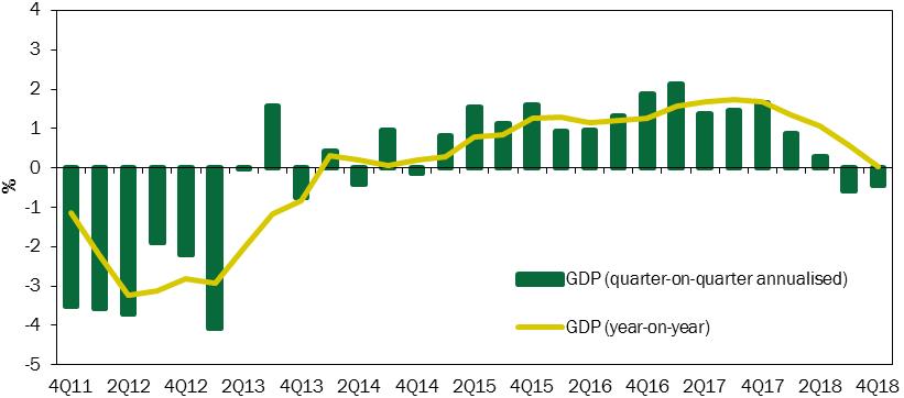
The Italian economy has lost momentum over the last year, recording an overall real GDP growth of 0.9 percent,
down from 1.7 percent in 2017. In fact, modest real GDP gains in the first two quarters were followed by slight declines in the third and fourth quarter.
Overall, the economic indicators available to date and nowcasting
estimates with internal models suggest that the contraction in economic activity has paused in the first quarter of 2019. In January, employment, industrial production, exports of goods and retail sales have shown a
considerable rebound. On the other hand, the business and consumer confidence indices have continued to fall in January and February, recovering only slightly in March in services and construction.
Companies’ expectations are cautious, particularly in the case of the manufacturing sector. In the face of
these developments in the scenario under unchanged legislation, the forecast of average GDP growth in real terms for 2019 stood at 0.1 percent (1.0 percent in the scenario of the most recent official document1). This estimate is affected by the negative carryover (-0.1 percentage points) from the quarterly data for 2018. Cyclical prospects are also
adversely affected by the current configuration of the exogenous forecasting variables, including a lower expected growth of world trade.
|
FIGURE I.1: GROSS DOMESTIC PRODUCT (percentage growth rate)
|
|
|
Source: ISTAT.
|
___
1 Update of the Macroeconomic
and Public Finance Framework, December 2018.
|
MINISTRY OF ECONOMY AND FINANCE
|
1
|
|
ECONOMIC AND FINANCIAL DOCUMENT - SECT. I STABILITY PROGRAMME
|
As regards nominal GDP, the estimate at unchanged legislation envisaged for 2019 stands at 1.2 percent. To
the dynamics highlighted above we must also add a marginal reduction of the GDP deflator, the increase of which drops from 1.1 to 1.0 percent in the presence of weak inflationary pressures.
It should be noted that the new forecast at unchanged legislation for 2019 is based on the expectation of a
gradual resumption of quarterly GDP growth that would rise to an annualised rate of 1.2 percent in the second half from just above zero in the first two quarters of the year.
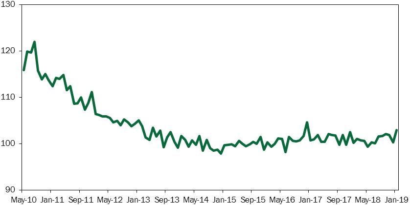
The slowdown in recent quarters was mainly due to the sharp decline in the growth of world trade and a fall
in industrial production in Europe, in particular in Germany. Exports of goods and services from Italy increased by only 1.9 percent in 2018 after having grown by 5.9 percent in real terms in 2017. The fall of exports
occurred at the beginning of 2018 and over the year resulted in a downward revision of companies’ investment programmes and to a decline in industrial production, which was however slightly more modest than that recorded
in Germany.
From the second quarter, these external factors were joined by a marked rise in yields on government bonds,
which was accompanied by greater caution among businesses and households. The growth of household consumption essentially halted starting from the second quarter, while gross fixed capital formation generally fell in the
second half of the year, so that its growth trend went from an average of 5.7 percent in the first half to only 0.9 percent in the second half of the year.
|
FIGURE I.2: RELATIVE INDUSTRIAL PRODUCTION INDEX, GERMANY VS ITALY
|
|
|
Source: MEF calculations on ISTAT and Destatis data.
|
|
2
|
MINISTRY OF ECONOMY AND FINANCE
|
|
I. OVERALL FRAMEWORK
|
|
I.2
|
MACROECONOMIC SCENARIO AND PUBLIC FINANCE TRENDS
|
The forecasts on the performance of world trade issued by major international organisations have also
recently suffered a continuous downward revision. The growth expectations for the main trading partners in Italy are positive, but they have a lower rate than 2018 and a lower drive from the manufacturing sector, also
due to uncertainty on the trade policies of the USA and China.
As regards domestic factors, before considering the most recent economic policy initiatives taken by the
Government, discussed within the policy scenario, the improvement of financial conditions should be noted. The yields on government bonds, although high in relation to the background data of the Italian economy,
decreased significantly with respect to the final months of 2018. There have also been positive developments in the stock market, which has recovered most of the losses recorded in the second half of 2018.
In this context, it should also be borne in mind that the most important expansionary measures laid down by
2019 Budget Law will begin to drive economic activity in the coming months. The delivery of the benefits envisaged by the Citizenship Income (RdC for its Italian acronym) began in April. This should provide a stimulus
to consumption of less well-off families, who have a higher than average propensity to consumption. Therefore, the impact on cyclical growth of household consumption is expected from the second quarter of this year.
Considering the delay with which the other main macroeconomic variables respond to the increase in consumption, the incremental stimulus to GDP growth will persist for several quarters, also influencing average GDP
growth in 2020. Overall, the RdC should raise real GDP growth by 0.2 percentage points both in 2019 and in 2020; the changes to the welfare system would have a neutral effect this year and would instead increase growth
by 0.1 percentage points in 20202.
The 2019 Budget Law also provides for more resources for public investment in comparison to last year, as
well as the creation of coordination and planning units for public investment. According to the most updated scenario at unchanged legislation of the general government’s accounts, in 2019 public investment will
increase by 5.2 percent. In the forecast, it was assumed that the stimulus from this increase would occur starting from the second quarter of the year. Overall, the increase provided for in the scenario based on
unchanged legislation should provide a contribution to real GDP of more than 0.1 percentage points.
This said, it must be emphasised that the GDP growth forecast for year 2019 is subject to downside risks,
linked in particular to the uncertainty surrounding international trade, the threat of protectionism, geopolitical factors and paradigm shifts in key industries such as the automotive and componentry sectors.
___
2 See the focus on the
macro characteristics and impacts of the two measures in Chapter II of this document.
|
MINISTRY OF ECONOMY AND FINANCE
|
3
|
|
ECONOMIC AND FINANCIAL DOCUMENT - SECT. I STABILITY PROGRAMME
|
|
TABLE I.1: SUMMARY OF MACROECONOMIC FRAMEWORK BASED ON UNCHANGED LEGISLATION (percentage variations, except where
otherwise indicated) (1)
|
|||||
|
|
2018
|
2019
|
2020
|
2021
|
2022
|
|
GDP
|
0.9
|
0.1
|
0.6
|
0.7
|
0.9
|
|
GDP deflator
|
0.8
|
1.0
|
1.9
|
1.7
|
1.5
|
|
Consumption deflator
|
1.1
|
1.0
|
2.3
|
1.8
|
1.5
|
|
Nominal GDP
|
1.7
|
1.2
|
2.6
|
2.5
|
2.4
|
|
Employment (FTEs) (2)
|
0.8
|
-0.2
|
0.2
|
0.5
|
0.6
|
|
Employment (labour force) (3)
|
0.8
|
-0.3
|
-0.1
|
0.5
|
0.6
|
|
Unemployment rate
|
10.6
|
11.0
|
11.2
|
10.9
|
10.6
|
|
Unemployment rate net of the activation effect (4)
|
10.6
|
10.5
|
9.7
|
9.3
|
9.0
|
|
Current account balance (balance in % of GDP)
|
2.6
|
2.6
|
2.5
|
2.5
|
2.5
|
|
(1) Discrepancies, if any, are due to rounding.
|
|||||
|
(2) Employment expressed in terms of Full-time equivalent units.
|
|||||
|
(3) Number of employees based on the sample survey of the Continuous Labour Force Survey (CLFS).
|
|||||
|
(4) Estimate of the unemployment rate net of the activation effect of the new labour force incentivised by
Citizenship Income.
|
|||||
Looking beyond the current year, the profile of real GDP growth is also revised downwards for the
2020-2021 period, albeit considerably less accentuated than for the year in progress. The path of nominal GDP falls significantly in comparison to the previous official forecast, which also reflects a lowering of the
deflator forecasts.
If the new forecasts are compared with those of the DEF 2018, the different configuration of exogenous
variables accounts for most of the downward revision. Within the exogenous variables, the less favourable growth prospects of the rest of the world and of international trade are the most decisive factor for the
worsening of the forecast, especially for 2019. The weighted exchange rate of the euro and the price of oil also have a negative effect, although only until 2020. From 2019 onwards the high level of the spread on government bonds negatively, and to an increasing extent, affects the downward revision.
The real GDP growth rate in 2022, forecast for the first time, is expected to be 0.9 percent. This
forecast takes account of the fact that the main international predictors envisage a deceleration of world growth on a three-four year horizon and that it is common practice to converge the GDP forecast toward the
potential GDP growth rate where there is a longer forecasting horizon3.
As regards nominal GDP, growth would accelerate from 1.2 percent in 2019 to 2.6 percent in 2020 and then
slow down slightly to 2.5 percent in 2021 and to 2.4 percent in 2022.
___
3 The main international
organisations estimate a potential Italian real GDP growth rate of between 0.5 (European Commission, forecast for 2020 in the Ageing Report 2018) and 0.8 percent (International Monetary Fund, Italy 2017 Article IV
Consultation). Matters relating to the estimation of potential GDP according to the Community methodology are discussed in paragraph III.2 of this document.
|
4
|
MINISTRY OF ECONOMY AND FINANCE
|
|
I. OVERALL FRAMEWORK
|
When reading the trend forecast one must take account of the fact that the unchanged legislation, as
amended by the 2019 Budget Law, provides for an increase in VAT rates in January 2020 and January 2021, as well as a slight increase of excise duties on fuels in January 2020. According to estimates obtained with
the Treasury’s econometric model (ITEM), the increase in indirect taxes would lead to lower GDP growth in real terms and a rise in inflation - both in terms of GDP deflator and in terms of consumer prices - with
respect to a scenario of no fiscal change. These impacts would be concentrated in the years 2020 and 2021, but would also persist to a lesser extent in 2022 through the ITEM structure of delays.
The macroeconomic forecast based on unchanged legislation was validated by the Parliamentary Budgetary
Office on 25 March 2019.
Regarding public finance forecast at unchanged legislation, the net borrowing forecasts for 2019-2022
have been revised in light of the new macro framework and new final data published by ISTAT4. In 2018, the general government balance
has recorded a deficit of 2.1 percent of GDP, down from 2.4 percent in 2017. The primary balance (i.e. excluding interest payments) stood at 1.6 percent of GDP, an improvement of 1.4 percent over 2017. Although the
estimate of the nominal deficit for 2018 is greater than indicated in the official December forecast (which was equal to ‑1.9 percent of GDP), the variation of the structural balance (i.e. adjusted for cyclical
factors and temporary measures) in 2018 is equal to zero, after having recorded a decrease of 0.4 percentage points in 2017.
In 2018, the debt-to-GDP ratio rose to 132.2 percent, from 131.4 percent in 2017. This trend is due to
the low growth of nominal GDP and, for a further 0.3 points, to the increase in the Treasury’s liquidity stock at year-end.
As regards 2019, the net borrowing at unchanged legislation is currently forecast at 2.4 percent of GDP
(2.0 percent of GDP in the Update presented in December). For 0.4 percentage points, the upward revision reflects the expected lower nominal growth and for 0.1 points, it reflects a different assessment of tax
refunds and compensations, while the block on two billion of public expenditure introduced by the Budget Law reduces the net borrowing by about 0.1 points. It is recalled that regulations envisage that the
expenditure in question may be authorised in the middle of the year only as a result of the check on the consistency of the evolution of public accounts with the policy scenario objective of 2 percent of GDP.
In 2019, the debt-to-GDP ratio is estimated at 132.8 percent of GDP, including privatisations proceeds
equal to 1 percent of GDP. This is due to the combined effect of an unfavourable differential between average implicit cost of debt financing and nominal growth and a drop in the primary surplus to 1.2 percent of
GDP, from 1.6 percent last year.
___
4 ISTAT, GDP and
general government net borrowing: update, April 9, 2019.
|
MINISTRY OF ECONOMY AND FINANCE
|
5
|
|
ECONOMIC AND FINANCIAL DOCUMENT - SECT. I STABILITY PROGRAMME
|
Over the 2020-2022 period, the public finance scenario based on unchanged legislation is characterised
by a decline in the general government deficit to 2 percent of GDP in 2020 and to 1.8 percent in 2021 and then close to 1.9 percent in 2022. In correspondence with these nominal balances, the structural deficit is
expected to widen to 0.1 percentage points in 2019, but compliance with the target in terms of structural balance would still be guaranteed considering the flexibility clause for exceptional events agreed at the
end of the year with the European Commission5. This would therefore improve by 0.4 points in 2020 and 0.2 points in 2021, and then
worsen by 0.1 points in 2022. The main reason for which the balances in both nominal and structural terms would worsen in 2022 is that the tax burden under unchanged legislation would be reduced by 0.2 percentage
points, while the interest expenditure as a ratio to GDP would rise to 3.9 percent in 2022 from 3.7 percent in 2021 because of the increase in expected yields on government securities in issue6.
The debt-to-GDP ratio in the scenario based on unchanged legislation would reduce from 132.8 percent in
2019 to 131.7 percent in 2020, and then settle at 129.6 percent in 2022. The debt rule would not be complied with either prospectively (forward-looking) or a posteriori (backward-looking), which highlights the
difficulty of achieving substantial reductions in the debt-to-GDP ratio in the presence of low nominal growth, relatively high real yields and a primary surplus that would remain slightly below 2 percent of GDP
even in the final year of the forecast.
This said the debt-to-GDP ratio forecasts must be contextualised in any case, since the implementation
of the public finance framework outlined here would probably lead to a drop in government bond yields, which would improve both the estimates of deficits and those relating to the debt-to-GDP ratio.
I.3 PUBLIC FINANCE POLICY SCENARIO
AND OFFICIAL MACROECONOMIC FORECAST
In the face of the trends described above, the policy scenario revises some capital revenue items
upwards and, at the same time, the refinancing of so-called unchanged policies.
Moreover, in conjunction with the publication of the present Stability Programme, the Government has
approved two decree-laws containing, respectively, measures to stimulate private investment and the territorial administrations (‘Growth’ Decree-Law) and measures to simplify the procedures for the approval of
public works and private construction projects (‘Unlock sites’ Decree-Law). The new measures are illustrated in detail in the National Reform
___
5 The agreement with
the European Commission considers exceptional expenditure for 0.18 percentage points of GDP, relating to interventions to protect against hydrogeological risk and safeguarding of viaducts, bridges and tunnels. The
flexibility clause must be applied to the structural adjustment required by the Stability and Growth Pact, which for 2019 is 0.6 percentage points of GDP according to the recommendation of the Council but is
reduced to 0.25 points in the presence of the cyclical conditions outlined in this document. See paragraph III.2 below.
6 As is common
practice, interest expenditure is projected based on forecasts of primary surpluses and maturing government bonds together with yield levels on the securities in issue calculated as forward rates based on the yield
curve observed in the period prior to closing the forecast.
|
6
|
MINISTRY OF ECONOMY AND FINANCE
|
|
I. OVERALL FRAMEWORK
|
Programme. The overall impact of the two measures on the economy is prudently estimated at 0.1 percentage points of additional real GDP growth in 2019. GDP growth in the policy scenario is therefore equal to 0.2 percent in real terms and 1.2 percent in nominal terms. In comparison to the forecast at unchanged legislation, gross fixed capital formation is the main component that explains the higher GDP growth.
The general government net borrowing objective for 2019 is confirmed to stand at 2.4 percent of GDP.
The structural balance will deteriorate by 0.1 percentage points, but this does not constitute a significant deviation in light of the economy’s cyclical conditions and the aforementioned clause for exceptional
events.
As regards the next three years, according to the policy scenario the general government net
borrowing is at 2.1 percent in 2020 and then 1.8 percent in 2021 and 1.5 percent in 2022. The structural balance is expected to improve by 0.2 percentage points of GDP in 2020 and 0.3 per year in 2021 and in
2022, down from -1.5 percent of GDP in 2019 to -0.8 percent in 2022, in line with a gradual convergence toward the structural balance.
The policy scenario reflects greater public investment in comparison to the scenario based on
unchanged legislation, to an increasing extent in the course of the three-year period (projections under unchanged legislation already envisage a considerable increase in public investment in 2020). Public
investment will rise from 2.1 percent of GDP in 2018 up to 2.6 percent of GDP in 2021 and 2022.
The existing legislation on tax measures is confirmed pending the definition of alternative measures
in the course of the next few months, in preparation for the 2020 Budget Law. Additional increases in revenue are also expected in 2021 and in 2022, which would arise mainly from measures to strengthen the fight
against tax evasion.
In addition to revenue measures, a programme for the comprehensive review of public expenditure will
also be implemented, with increasing effects over time.
|
TABLE I.2: SUMMARY OF MACROECONOMIC FRAMEWORK BASED ON POLICY
SCENARIO (percentage variations, except where otherwise indicated) (1)
|
|||||
|
|
2018
|
2019
|
2020
|
2021
|
2022
|
|
GDP
|
0.9
|
0.2
|
0.8
|
0.8
|
0.8
|
|
GDP deflator
|
0.8
|
1.0
|
2.0
|
1.8
|
1.6
|
|
Consumption deflator
|
1.1
|
1.0
|
2.3
|
1.9
|
1.6
|
|
Nominal GDP
|
1.7
|
1.2
|
2.8
|
2.6
|
2.3
|
|
Employment FTEs (2)
|
0.8
|
-0.1
|
0.3
|
0.6
|
0.5
|
|
Employment (labour force) (3)
|
0.8
|
-0.2
|
0.1
|
0.6
|
0.6
|
|
Unemployment rate
|
10.6
|
11.0
|
11.1
|
10.7
|
10.4
|
|
Unemployment rate net of the activation effect (4)
|
10.6
|
10.5
|
9.6
|
9.0
|
8.8
|
|
Current account balance (balance in percent of GDP)
|
2.6
|
2.5
|
2.4
|
2.4
|
2.4
|
|
(1) Possible inaccuracies from rounding.
|
|||||
|
(2) Employment expressed in terms of Full-time equivalent units.
|
|||||
|
(3) Number of employees based on the sample survey of the Continuous Labour Force Survey (CLFS).
(4) Estimate of the unemployment rate net of the activation effect of the new labour force incentivised by
Citizenship Income.
|
|||||
|
MINISTRY OF ECONOMY AND FINANCE
|
7
|
|
ECONOMIC AND FINANCIAL DOCUMENT - SECT. I STABILITY PROGRAMME
|
The streamlining of procedures for public contracts and private construction and the highest level
of public investment in the policy scenario, even in the presence of financial hedging measures, ensure a positive differential of GDP growth in comparison to the scenario under unchanged legislation equal to
0.2 percentage points in 2020 and 0.1 points in 2021. GDP growth would only be lower than the forecast at unchanged legislation by 0.1 percentage points in the last year of the forecast, 2022, due to a more
challenging deficit target.
As regards compliance with the national budget rules and the Stability and Growth Pact (SGP), it is
worth noting the deviation recorded in 2018, the year in which, as has been shown above, the structural balance remained unchanged compared to an improvement of 0.3 percentage points that the previous
Government had negotiated with the European Commission7. With regard to 2019, considering that the Government’s forecasts
estimate a growth lower than the potential growth and a negative output gap by over 1.5 percentage points (-1.7 to be precise), the improvement in the structural balance required by the SGP would be equal to
0.25 percentage points. Subtracting the clause of 0.18 points that was granted for exceptional events from this value, one obtains a required improvement of 0.07 points. With respect to this benchmark, the
forecast variation in the structural balance of 2019 does not significantly deviate.
Finally, as described in detail in paragraph III.2 of this document, the policy scenario objectives
outlined here are in line with the dictates of the SGP while generally aiming for more contained improvements in the structural balance in comparison to a literal interpretation of the rules.
The debt-to-GDP ratio under the policy scenario will rise from 132.2 percent in 2018 to 132.6
percent at the end of 2019. A gradual descent is instead expected for the next three years, to 131.3 percent in 2020, 130.2 percent in 2021 and finally to 128.9 percent in 2022.
The substantial compliance of the public finance policy scenario outlined here with the preventive
arm of the SGP will constitute a significant factor for the evaluation of Italy’s compliance with the debt rule, which the European Commission will carry out based on the final estimates for 2018.
___
7 The preventive
arm of the SGP would have required the structural balance to improve by 0.6 percentage points, given the cyclical conditions in which Italy found itself in 2018. However, in 2017 the European Commission decided
to apply a margin of discretion in formulating its recommendation for the Council Recommendation concerning 2018. This resulted in the indication of an improvement of 0.3 percent for 2018.
|
8
|
MINISTRY OF ECONOMY AND FINANCE
|
|
I. OVERALL FRAMEWORK
|
|
TABLE I.3: PUBLIC FINANCE INDICATORS (as percentage of GDP) (1)
|
|||||||
|
2017
|
2018
|
2019
|
2020
|
2021
|
2022
|
||
|
POLICY SCENARIO
|
|||||||
|
Net borrowing
|
-2.4
|
-2.1
|
-2.4
|
-2.1
|
-1.8
|
-1.5
|
|
|
Primary balance
|
1.4
|
1.6
|
1.2
|
1.5
|
1.9
|
2.3
|
|
|
Interest
|
3.8
|
3.7
|
3.6
|
3.6
|
3.7
|
3.8
|
|
|
Structural net borrowing (2)
|
-1.4
|
-1.4
|
-1.5
|
-1.4
|
-1.1
|
-0.8
|
|
|
Variation in the structural balance
|
-0.4
|
0.0
|
-0.1
|
0.2
|
0.3
|
0.3
|
|
|
Public debt (gross of support) (3)
|
131.4
|
132.2
|
132.6
|
131.3
|
130.2
|
128.9
|
|
|
Public debt (net of support) (3)
|
128.0
|
128.8
|
129.4
|
128.1
|
127.2
|
125.9
|
|
|
Proceeds from privatisation
|
0.0
|
0.0
|
1.0
|
0.3
|
0.0
|
0.0
|
|
|
SCENARIO BASED ON UNCHANGED LEGISLATION
|
|||||||
|
Net borrowing
|
-2.4
|
-2.1
|
-2.4
|
-2.0
|
-1.8
|
-1.9
|
|
|
Primary balance
|
1.4
|
1.6
|
1.2
|
1.6
|
1.9
|
2.0
|
|
|
Interest
|
3.8
|
3.7
|
3.6
|
3.6
|
3.7
|
3.9
|
|
|
Structural net borrowing (2)
|
-1.4
|
-1.5
|
-1.6
|
-1.2
|
-1.0
|
-1.2
|
|
|
Variation in the structural balance
|
-0.4
|
0.0
|
-0.1
|
0.4
|
0.2
|
-0.2
|
|
|
Public debt (gross of support) (3)
|
131.4
|
132.2
|
132.8
|
131.7
|
130.6
|
129.6
|
|
|
Public debt (net of support) (3)
|
128.0
|
128.8
|
129.5
|
128.5
|
127.6
|
126.6
|
|
|
MEMO: Update of the Public Finance Framework (December 2018)
|
|||||||
|
Net borrowing based on unchanged legislation
|
-1.9
|
-2.0
|
-1.8
|
-1.5
|
|||
|
Structural net borrowing (2)
|
-1.1
|
-1.3
|
-1.2
|
-1.0
|
|||
|
Public debt (4)
|
131.7
|
130.7
|
129.2
|
128.2
|
|||
|
MEMO: Update of DEF 2018 (September 2018)
|
|||||||
|
Net borrowing
|
-2.4
|
-1.8
|
-2.4
|
-2.1
|
-1.8
|
||
|
Primary balance
|
1.4
|
1.8
|
1.3
|
1.7
|
2.1
|
||
|
Interest
|
3.8
|
3.6
|
3.7
|
3.8
|
3.9
|
||
|
Structural net borrowing (2)
|
-1.1
|
-0.9
|
-1.7
|
-1.7
|
-1.7
|
||
|
Variation in the structural balance
|
-0.2
|
0.2
|
-0.8
|
0.0
|
0.0
|
||
|
Public debt (5)
|
131.2
|
130.9
|
130.0
|
128.1
|
126.7
|
||
|
Nominal GDP based on unchanged legislation (absolute val. x 1,000)
|
1727.4
|
1757.0
|
1777.9
|
1823.3
|
1868.9
|
1914.5
|
|
|
Nominal GDP based on policy scenario (absolute val. x 1,000)
|
1727.4
|
1757.0
|
1778.6
|
1828.4
|
1875.5
|
1918.9
|
|
|
(1) Discrepancies, if any, are due to rounding.
(2) Net of one-offs and the cyclical component.
(3) Gross or net of Italy’s relevant shares of the loans to Member States of the EMU, bilateral or
through the EFSF, and of the contribution to the capital of the ESM. At the end of 2018, the amount of these shares was equal to approximately 58.2 billion, of which 43.9 billion for bilateral loans
and through the EFSF and 14.3 billion for the ESM programme (see Bank of Italy, ‘Statistical Bulletin - The Public Finances, borrowing requirement and debt’ of March 15, 2019). The estimates consider
proceeds from privatisation and other financial income equal to 1 percent of GDP in 2019, 0.3 percent of GDP in 2020 and 0 in subsequent years. Moreover, a reduction of the MEF’s liquidities of 0.1
percent of GDP for each year from 2019 to 2021 is assumed. The interest rates scenario used for the estimates are based on the implicit forecasts resulting from the forward rates on Italian government
bonds of the period for the compilation of the present document.
(4) Gross of Italy’s relevant shares of the loans to Member States of the EMU, bilateral or through
the EFSF, and of the contribution to the capital of the ESM. The estimates consider proceeds from privatisation and further savings intended to fund depreciation equal to 1.0 percent of GDP in 2019
and to 0.3 percent of GDP in 2020.
(5) Gross of Italy’s relevant shares of the loans to Member States of the EMU, bilateral or through
the EFSF, and of the contribution to the capital of the ESM. The estimates consider proceeds from privatisation and further savings intended to fund depreciation equal to 0.3 percent of GDP in 2019
and in 2020.
|
|||||||
|
MINISTRY OF ECONOMY AND FINANCE
|
9
|
|
ECONOMIC AND FINANCIAL DOCUMENT - SECT. I STABILITY PROGRAMME
|
To complete the budgetary measures, the Government confirms the draft laws indicated in the
previous planning document, and indicates the following draft laws connected to the public finance measures for 2020:
| • |
Draft law to delegate to the Government for the adoption of provisions for fighting violence at sporting events (Chamber Act
1603-TER);
|
| • |
Draft law containing delegations to the Government for the improvement of Public Administrations (Senate Act 1122).
|
|
10
|
MINISTRY OF ECONOMY AND FINANCE
|
II. MACROECONOMIC FRAMEWORK
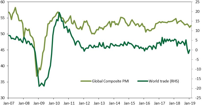
II.1 THE INTERNATIONAL ECONOMYIn 2018, the trend of the world economy was characterized by a slowdown in growth mainly due to a lower
dynamism in international trade, which had instead been a powerful driver in the previous year.
The slowdown was triggered mainly by the intensification of trade tensions between the United States and
China, which, together with the emergence of geopolitical tensions in other important countries and the increased socio-economic instability within some emerging countries, strongly influenced
business and financial markets confidence, leading to the adoption of wait-and-see strategies for investment programmes amidst growing uncertainty. In the second semester of last year, the effects of
these developments began to spread to domestic demand in the more developed countries through a significant fall in investment and lower consumer spending. As a result, manufacturing stalled,
especially the production of investment goods, with economies still highly specialized in the industrial sector, such as in the case of Germany, proving to be particularly vulnerable.
|
FIGURE II.1: GLOBAL COMPOSITE PMI AND WORLD TRADE
(index; % var. y/y RHS)
|
|
|
Source: CPB and Markit.
|
|
MINISTRY OF ECONOMY AND FINANCE
|
11
|
|
ECONOMIC AND FINANCIAL DOCUMENT - SECT. I STABILITY PROGRAMME
|
The outlook for manufacturing remains weak for the current year as well; the global composite PMI index,
excluding the euro zone, has continued to record a contraction of production in manufacturing, especially in those countries whose economic cycle now appears to be mature. The services sector seems
more resilient, although it has moderated compared to last year and in recent months has been just above the expansion threshold.
According to the latest official estimates of the International Monetary Fund, in 2018 world growth stopped
at 3.6 percent, down from the 3.8 percent in the previous year, bearing negative effects on the current year due to the increased slowdown in the second semester of 2018. As a consequence, the
updated 2019 projections, the result of a series of downward revisions, predict a slower expansion, of 3.3 percent, mainly tied to the weakened cycle of advanced countries (1.8 percent, down from
2.2 percent in 2018).
In the last two years, the US economy has benefited from the effects of a major tax stimulus that started,
however, at an advanced stage of the expansionary cycle. At any rate, the first signs of weakening appeared at the end of last year, pointing to the risk of an economic cool down in 2019 for the
United States, which is burdened with a heavy public debt. In 2018, the US economy continued to expand at a sustained pace of 2.9 percent, very close to the 3 percent government target, thanks to
robust investment and increased consumption, which benefited from an excellent labour market and a stable unemployment rate, around 4 percent, at its historical minimum. The pressure from inflation
remained substantially low as well, thanks to moderate energy prices, leading consumer inflation to around 1.7 percent at year’s end. However, the pace of growth slowed down in the second half of
2018, giving less momentum to current year prospects; in Q4 2018, the GDP grew by 2.2 percent on an annual basis, slightly below expectations and decelerating in comparison to the previous quarters
(3.4 percent in 3Q and 4.2 percent in 2Q).
Accordingly, the IMF predicts that this year’s growth of 2.3 percent will slow down even further to 1.9 percent in 2020. These
expectations are justified mainly by the weakening of fiscal policy stimulus over the past two years; the US Congressional Budget Office (CBO) predicts a 0.8 pp growth rate slowdown of the US
economy this year and another slowdown, by 0.6 pp, in the following year; the weakening factors being identified in reduced private investment in conjunction with the greatly reduced federal
spending foreseen by the legislation in force in the last quarter of last year. The CBO also estimates that, from last year, the US economy has been growing above its potential, causing salaries,
prices and interest rates to rise.
On the other hand, the US economy’s growth potential could benefit from the repatriation of retained
earnings of American multinationals stimulated by the tax reform; compared to the previous year, in 2018 there was a fall in profits reinvested by American multinationals of over 360 billion
dollars, which was the main cause for the broad contraction of FDI flows to advanced economies in the same period (-40 percent)1. Actual gain in terms of growth potential expansion
___
1 UNCTAD ‘Investment Trade
Monitor’, January 2019.
|
12
|
MINISTRY OF ECONOMY AND FINANCE
|
|
II. MACROECONOMIC FRAMEWORK
|
will depend in any case on how these multinationals will decide to employ the repatriated earnings on national territory.
The concerns triggered on the financial markets by bullish expectations for interest rates related to the
sustainability of the high federal public debt were calmed by the FED’s decision to reconsider the normalization of monetary policy; departing from the two policy-rate increases initially planned
for the current year, the consensus within the FOMC (Federal Open Market Committee, which decides monetary policy) has shifted towards maintaining the current federal funds rate at 2.25-2.5
percent. The FOMC also announced that its balance sheet would be normalized by next September, reaching over 3.500 billion dollars.
Still in terms of advanced economies, Europe is also showing even greater signs of an economic slowdown:
GDP growth stalled at 1.8 percent in 2018, against 2.3 percent in 2017. Starting from early last year, there has been a progressive deterioration in the performance of the main euro zone
economies, initially triggered by the absence of impetus towards foreign trade and spreading to domestic demand over the months, especially as regards private investment. Since the downturn
concerned mainly the manufacturing industry, while the service sector showed greater resilience, countries such as Germany and Italy, whose economies are industry driven, were the most affected.
Business confidence and investment choices were also greatly influenced by the uncertainty caused by the United Kingdom's exit from the EU, the developments of which are still being defined.
As for the monetary policy, the European Central Bank (ECB) budget expansion phase, trough the
Quantitative Easing (QE) programme, concluded with the end of 2018, though the ECB confirmed its commitment to reinvest the capital repaid on the securities maturing for an extended period of
time, i.e. even after the first policy rate increase. The ECB responded to signs of a cyclical weakening and an inflation rate that persists under the two percent target, especially in the
‘underlying’ component (i.e. excluding fresh food and energy), by changing its forward guidance (indications to markets about the timing of a possible rate hike) and announcing new long-term
refinancing operations. According to the Governing Council’s latest statements, there will be no increase in policy rates before the end of this year and for as long as a substantial degree of
monetary accommodation is deemed necessary. Furthermore, starting September 2019 and every three months until March 2021, support for growth will also be guaranteed through new longer-term
targeted refinancing operations (TLTRO III) with two-year maturity, aimed at preserving favourable bank credit conditions.
The latest business confidence surveys show that the euro zone will continue to experience modest growth
in the short term. PMI surveys indeed report a contraction of the manufacturing sector in the main EU countries in the first three months of 2019, which seems set to continue into the next quarter
and is no longer duly offset by the solidity of the tertiary sector. The most worrying aspect is the impact that fewer orders are beginning to have on the investment plans and employment decisions
made by companies.
On the other hand, considering that in recent months performance has been affected by specific and
potentially temporary factors, such as the shock to the automotive industry caused by the revised anti-pollution regulations and social unrest in France, and provided that no new external factors
come up, European
|
MINISTRY OF ECONOMY AND FINANCE
|
13
|
|
ECONOMIC AND FINANCIAL DOCUMENT - SECT. I STABILITY PROGRAMME
|
economies could prove more resilient in the upcoming months. An example of this is Germany, whose
automotive market took quite a hit recently, but has a fundamentally healthy economy: after several months of negative figures, the IFO business survey, despite confirming the weakness of the
manufacturing industry, also detected room for improvement and recovery in the months to come, with renewed improvements in business expectations. All in all, modest growth is expected for the
current year as well, along with the gradual stabilization of the cycle in the subsequent years. The IMF estimates moderate euro zone growth (1.3 percent) in the year underway and a slight
recovery in 2020 (1.5 percent).
The slowdown of the main Asian economies continues to exert pressure on global
growth in 2019. Observers have been expecting China’s gradual economic cool down for quite some time now. China’s GDP has indeed shown a gradual deceleration in 2018, more so in the second
semester, leading to a 6.6 percent annual growth down from 6.8 percent in 2017 (the National Institute of Statistics revised this result down from the initial 6.9 percent). This is the lowest
annual average growth rate since 1990, albeit slightly higher than the target set by the Government at the beginning of the year (6.5 percent). The worsening trade relations with the United
States, involving gradually higher duties on imported goods, although not as high as initially announced, is undoubtedly partially responsible for these results.
In addition, domestic demand and especially investment were affected by a
restrictive debt-reduction tax policy, more rigorous checks over the approval process of local public investment projects, and a squeeze on the shadow banking system, which is a group of
unofficial financial intermediaries highly exposed to credit risks. All these measures depressed internal demand, leading the Central Bank to intervene in early 2019 to rebalance the market and
provide credit to the private sector through two channels: the strong injection of liquidity into the banking system for the record amount of 560 billion yuan (83 billion dollars); and cutting
banks’ compulsory reserve ratios by 100 basis points for the fifth straight time in the past twelve months, which should have freed up over one hundred billion dollars for new loans.
China’s fiscal policy will also guarantee support to the economy; Premier Li Keqiang
announced at the opening of the National People's Congress that tax cuts and support for employment (under pressure due to the transformation of production processes) will be two of the main
pillars of the economic policy strategies for the near future. The goal is to reduce the tax burden on businesses in addition to cutting value added tax. Local authorities will also contribute
by issuing new debt for infrastructure financing. Overall, the main international forecasters remain positive, with gradual moderation of growth towards sustainable levels in the medium to long
term, achievable in part thanks to China’s gradual wage alignment.
As for Japan, whose economy had regained momentum in 2017, closing with an
acceleration of 0.8 pp as compared to the previous year, it too recorded a slowdown in GDP growth, which is estimated to have stalled at 0.8 percent in 2018, under the burden of major natural
disasters that affected economic activity in the second part of the year. Japan’s economy is also amongst those most affected by international trade tensions; since the autumn of last year, the
dip in
|
14
|
MINISTRY OF ECONOMY AND FINANCE
|
|
II.
MACROECONOMIC FRAMEWORK
|
foreign demand by China has been damaging markedly the dynamics of Japanese exports with significant
repercussions on industrial activity.
According to the most recent surveys on the confidence climate of Japanese
businesses, operators are increasingly concerned about the reduction in orders from China, which is leading to an overall slowdown in investment, much of which has been either postponed or
downsized, especially in the fields of robotics and industrial machinery. Looking ahead, fears are rising that the slowdown may also affect the coming months, when fiscal policies could also
have a negative impact on the economic cycle, given the planned increase in consumption taxes that could lead to a reduction in domestic demand too.
Based on the above, both the Government and the Central Bank have revised downwards
their growth expectations for the current year, though without contemplating the risk of recession. On the monetary policy front, this has meant confirmation of a policy that is still
accommodative, with unchanged rates and the commitment to additional measures according to the demands of economic trends. On the fiscal policy front, the Government’s draft budget for the
current year includes the undertaking of expansionary policies, postponing the primary surplus target to 2025; for the years 2019-2020, in fact, the deficit and macroeconomic impact of the
consumption tax increase scheduled for October will be substantially neutralized by the decision to use half of the increased revenue for new spending programmes. The overall expectations for
the current year are therefore favourable, as domestic demand should contribute to a new growth rate acceleration of around 1 percent, thanks to new tax breaks and wage increases that were
already implemented in the second half of 2018 due to the reduced production capacity.
Therefore, at the global level, fiscal policy strategies will differ depending on
the specific economic conditions of individual countries, but no restrictive measures of such magnitude as to jeopardize economic expansion are expected. In the United States too, where last
year’s tax reform more than exhausted the available fiscal space, a budget policy is predicted2 that may prove
moderately restrictive only in the last part of the year due to a reduction in federal funding under current legislation. The current Government will focus on preserving the margins for fiscal
manoeuvres that are still available for the beginning of next year, in order to use them to fuel the upcoming 2020 presidential campaign.
On the other hand, the monetary policy should also prove to be accommodative
overall, considering the restructuring of the FED strategy and the confirmation of the current stance by all the other main central banks. This also eases the pressure on emerging countries,
whose economies were strongly affected by the appreciation of the dollar in 2018 triggered by the increases in policy rates established by the FED. The accommodating attitude of the central
banks also seems to have had a strong stabilizing effect on the markets, the volatility of which remains essentially limited, despite the negative signals of macroeconomic indicators.
___
2
CBO, ‘The Budget and Economic Outlook: 2019 to 2029’, January 2019.
|
MINISTRY OF ECONOMY AND FINANCE
|
15
|
|
ECONOMIC AND FINANCIAL DOCUMENT - SECT. I STABILITY PROGRAMME
|
|
FIGURE II.2: PERFORMANCE OF 10 YEAR GOVERNMENT SECURITIES
|
 |
|
Source: Bloomberg.
|
An accommodative monetary policy is also allowed by low inflation rates in almost
all the advanced economies at the beginning of the year, due to a significant cost reduction of energy goods that occurred late in the previous year, and as a reflection of the overall
economic slowdown. In almost all countries, in fact, consumer inflation stands at levels far removed from the targets of the main central banks. The only exceptions are the United States and
the United Kingdom, where consumer price growth is averaging above 2 percent. On the other hand, wage growth remains modest in all the advanced economies, despite the fact that in many of
these economies, first and foremost the United States, the labour market has achieved positive results at all-time highs. The same goes for emerging countries, where, because of the global
economic slowdown, inflation fell sharply to its lowest levels in the past ten years after peaking no later than last October. This triggered expectations that central banks would lower policy
rates, primarily in countries like Russia and Mexico, after the increases introduced in the autumn of last year in conjunction with the peak in inflation and some localized depreciation.
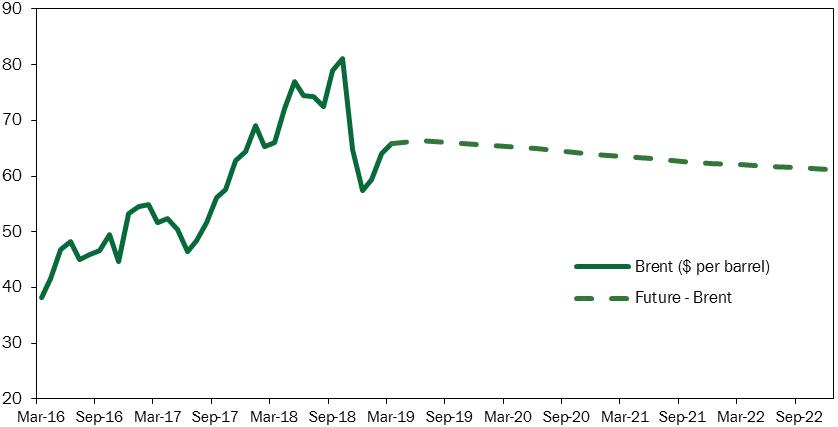
As for the energy products and commodities market, in 2018, after an initial rise
in fuel prices, there was a marked deceleration, more so late in the year, due to multiple factors. On the one hand, pressure came from supply factors such as the temporary shield granted by
the United States to eight major importers of crude oil in connection to the sanctions imposed on Iran and the record US production of shale oil; on the other, there was the effect on global
demand of the economic slowdown. However, since early this year, there has been a renewed upward trend, mainly due to the supply restrictions brought about by the Venezuelan crisis and the
continuing tensions with Iran, whose temporary shield from sanctions will expire on 4 May.
|
16
|
MINISTRY OF ECONOMY AND FINANCE
|
|
II. MACROECONOMIC FRAMEWORK
|
|
FIGURE II.3: BRENT AND FUTURES PRICE
|
|
|
Source: Thomson Reuters Datastream.
|
The tensions that had affected the financial markets in 2018, especially until
the autumn of last year, abated significantly after the recent monetary policy announcements by the central banks of the main advanced countries, which, as mentioned, took a much more
gradual path of monetary normalization. This provided breathing space for emerging countries as well, whose yields on sovereign debt securities and related spreads with advanced countries
are gradually retreating after the peaks recorded in late 2018. Following the dip, the rate curves flattened out; in particular, the US curve now shows a slightly negative trend, which is
normally indicative of recession. In consideration of the substantial stability of financial volatility indicators, it would seem that at present the markets are more focused on an
accommodative monetary policy stance rather than on the risk of a much more marked slowdown or recession.
Forecast risks
In recent months, there has been a progressive deterioration in the
expectations of international observers, with an increasingly downward trend in risk scenarios. On the other hand, the most recent signals from the economic seem to paint a less grim picture
than that predicted late last year. All in all, there is a situation of uncertainty such as to render future risk scenarios more balanced.
The uncertainty over the evolution of international trade continues to bear on
business decisions of investment and production. Whereas 2019 began with signs of relaxation between the United States and China, there are fears of worsening trade relations between America
and Europe in the near future.
The expectations of weaker global demand are also influenced by concerns of a
faster than expected slowdown of the main world economies, namely the United States, China and Europe. However, China’s latest macroeconomic data show resilient domestic demand and a
reorganization of trade flows in exports in Asian,
|
MINISTRY OF ECONOMY AND FINANCE
|
17
|
|
ECONOMIC AND FINANCIAL DOCUMENT - SECT. I STABILITY PROGRAMME
|
which could lead to greater stabilization. Chinese GDP dynamics should also benefit from clearly
favourable monetary and fiscal policies.
As for the slowdown in the euro zone, there are prospects of a moderation in
growth but the risks of an actual recession appear to be relatively limited; in the event of recovery in international trade thanks to progress in international negotiations, the recovery
in foreign demand could generate renewed support for European economies that have been most penalized so far. On the other hand, the monetary policy instruments still effectively available
to the ECB are at present much more limited than those available at the time of the sovereign debt crisis.
In terms of financial markets, the ups and downs recorded at the end of 2018
calmed down after the announcements of the ECB and especially of the FED. However, if the current economic slowdown should prove to be worse than currently expected or unforeseen events
were to lead to a sudden change in expectations, this could trigger sharp and dangerous corrections on financial markets.
II.2 THE ITALIAN ECONOMY
In 2018, the Italian economy grew by 0.9 percent, slowing down compared to
the previous year. After modest growth in the first quarter of 2018 (0.2 percent Q/Q), the GDP slowed further in the second quarter (0.1 percent Q/Q) and experienced slightly negative
growth in the second half of the year (-0.1 percent Q/Q in the third and fourth quarters). Domestic demand net of inventories continued to expand, albeit at lower rates than in 2017, while
inventories made a zero contribution. On the other hand, net exports subtracted 0.1 percentage points from growth due to global trade tensions.
In further detail, growth in private consumption more than halved (0.6
percent down from 1.5 percent), despite the dynamic trend of real disposable income driven by renewed contracts in the public sector and favourable credit eligibility conditions. Indeed,
the propensity to save increased over the year, reaching a peak in 2Q18 (8.5 percent up from 7.8 in 1Q18) and then gradually fell to 7.6 percent in 4Q18. On average, the propensity to save
stood at 8.0 percent, lower than the average of the last 10 years (9.0 percent). The slowdown in consumption may have been influenced by a reduction in wealth, with a contraction of around
130 billion in 4Q18 compared to 3Q18; empirical evidence shows that changes in financial wealth have an impact on household consumption3.
The wealth position of households remains solid; household debt in the third
quarter of 2018 was stable at 61.3 percent of disposable income, well below the euro zone average (94.8 percent)4.
Debt sustainability was also favoured by continuing low interest rates.
___
3
In particular, low propensity for consumption is more affected by a decline or increase in financial wealth than changes in real wealth. See, for example, A. Bassanetti & F. Zollino
(2010) The Effects of Housing and Financial Wealth on Personal Consumption: Aggregate Evidence for Italian Households. In: de Bandt O., Knetsch T., Peñalosa J., Zollino F. (eds) Housing
Markets in Europe. Springer, Berlin, Heidelberg.
4
Bank of Italy, Economic Bulletin, January 2019.
|
18
|
MINISTRY OF ECONOMY AND FINANCE
|
|
II. MACROECONOMIC FRAMEWORK
|
As for the type of spending, the growth in consumption of goods equalled
that of services (0.7 percent). Spending on durable goods slowed down while on semi-durable goods it grew more than the previous year. Non-durable goods were also down compared to the
previous year due to the higher pressure of inflation.
Investment continued to expand (3.4 percent), thanks to the average
performance recorded in the first part of the year. In contrast to the previous years, the contribution of the transport vehicles component was greatly reduced following the contraction
of the car market, which had driven the recovery of previous years. The Italian car and components industry, which engages 250.000 workers (directly and indirectly) and almost 6000
companies5, recorded a drop in production in 2018 compared to the previous year (‑3.4 percent), as well
as in turnover and number of orders (-2.1 and -2.4 percent respectively).
Investment in machinery slowed down compared to 2017. As to the
construction industry, there was an acceleration compared to 2017; investment in construction was driven by housing, while the increase in infrastructure investment was modest.
Investment in housing was in turn driven by the home renovation business, which now accounts for 37 percent of construction investment6.
As for the real estate market, housing prices were back down. The most
recent surveys7 confirm that quotations have continued to fall in the fourth quarter of 2018 (-0.2
percent) and are 0.6 percent lower than the corresponding period of 2017. Overall, the prices of existing houses fell by 1.0 percent in 2018, while those of new homes increased by 1.0
percent8. Real estate sales, probably positively affected by the price reduction, showed a simultaneous
recovery during 2018.
The construction industry, especially of real estate, continues to be an
important driver of economic recovery, in part due to its positive influence on consumption and employment. Furthermore, the trend in real estate prices has a direct effect on household
wealth. Data on non-financial assets show that houses constitute almost the totality of real household wealth9;
a recovery in prices could have a favourable effect on consumption.
Foreign demand, on the other hand, was weakened by the slowdown in world
trade due to tensions caused by stricter import duties. After a sharp decline in 1Q18, probably linked to the uncertainty deriving from the announcement of duties, exports returned above
zero but did not reach the peaks of the previous year. Imports also slowed down, following the weakening of domestic demand and of the industrial production cycle in particular.
On the supply side, the manufacturing industry continued to grow but at
decidedly lower rates (2.1 percent down from 3.6 percent in 2017). In 2018, the
___
5
Source: ANFIA.
6
ANCE Report http://www.ance.it/docs/docDownload.aspx?id=48610
7 See: ISTAT, ‘Home prices’, April 2018 and Bank of Italy,
‘Economic Bulletin’, April 2018.
8
ISTAT, https://www.istat.it/it/archivio/228988
9 In 2017, real estate assets owned by households accounted for over 92 percent of the total real estate value, of which 81
percent used as homes or second homes. The decline in house prices has led to a reduction in the value of housing wealth (-1.4 percent annual average over the period 2011-2017). However,
this trend is slowing down: -0.8 percent in 2017 down from -1.3 percent in 2016. ISTAT, ‘Non-financial assets of institutional sectors’, March 2019.
|
MINISTRY OF ECONOMY AND FINANCE
|
19
|
|
ECONOMIC AND FINANCIAL DOCUMENT - SECT. I STABILITY PROGRAMME
|
industrial production index (adjusted for calendar effects) show a marked slowdown from 3.6
percent, registered in 2017, to 0.8 percent. The different sectors show heterogeneous trends; even though they decelerated, non-durable capital goods and consumer goods still recorded
positive performances, while the production of durable intermediate and consumer goods decreased. The automotive and car components sector recorded a sharp drop in production compared to
the previous year. The construction sector is gradually improving, however growth is still weak (1.7 percent). The agriculture value added growth is back in positive territory (however,
this sector has limited effect on the GDP).
The services industry proved to be more resilient than manufacturing over
the year, but it too slowed down; growth in value added more than halved in 2018 compared to the previous year (0.6 percent compared to 1.4 percent). However, the various sectors showed
uneven trends. In the sectors of trade, accommodation and restaurants, transport and storage and real estate, growth remained positive (1.9 and 1.6 percent, respectively), while the
value added of finance, insurance, information and communication services fell back below zero (-1.3 and -2.7 percent, respectively); professional activities were only just above zero
(0.4 percent).
As to non-financial companies, the fall in profit share (defined by the
ratio between gross operating profit and value added) continued, albeit gradually, in 2018, reaching a value of 41.6 (down from 42.7 in 2017 and 43.3 in 2016). The latest data published
by the Bank of Italy for the third quarter of 2018 indicate that corporate debt as a percentage of GDP has fallen further, standing at 70.9 percent (down from 71.1 percent at the end of
June 2018)10.
The positive trend of the labour market continued in the first half of 2018
and then partially reversed in the second half of the year. Overall, employment growth, as recorded by the national accounts, stood at 0.9 percent, driven by employee numbers, whereas
the numbers of self-employed workers continued to fall for the eighth consecutive year. Hours worked increased by 1.1 percent, with hours worked per-capita increasing by 0.2 percent,
after the drop of the previous year.
Based on the results of the workforce survey, employment grew by 0.8
percent. The employment rate reached 58.5 percent, only 0.1 point off the peak of 2008. The increase was driven by dependent employment (1.2 percent), in turn driven exclusively by
temporary employment, while permanent employment was down for the first time in four years (-0.7 percent). In terms of hours of work, full-time employment increased and there was a
slight reduction in part-time. Involuntary part-time employment continued to increase, however (5.0 percent), up to 64.1 percent of total part-time employment. Improvements in the labour
market were reflected in the fall in unemployment (to 10.6 down from 11.2 percent). Another positive factor was the decline in the unemployed not seeking employment (-0.9 percent) and
those who no longer seek employment (-11.5 percent).
After the moderation of recent years, per capita incomes
returned to growth (2.0 percent up from 0.3 percent in 2017) due to renewed contracts in many
___
10
Bank of Italy, Economic Bulletin, January 2019.
|
20
|
MINISTRY OF ECONOMY AND FINANCE
|
|
II. MACROECONOMIC FRAMEWORK
|
sectors, including the public sector, and the gradual depletion of the tax relief schemes
introduced in 2015. Unit labour cost showed a significant recovery (1.9 percent up from -0.5 percent in 2017) thanks to the substantial stability of labour productivity.
Inflation remained substantially unchanged compared to the previous year
(1.2 percent compared to 1.3 percent), still driven by the volatile components; the underlying component was in fact more limited and slowed slightly compared to the previous year (0.7
percent down from 0.8 percent). Domestic inflation, however, measured by the GDP deflator, accelerated slightly (0.8 percent up from 0.4 percent) due to renewed PA contracts and
payments of arrears.
Foreign
trade
During 2018, the profound change in the international economic situation
was largely related to the further tightening of trade policies, a phenomenon that has been underway since 2012. The crisis of confidence triggered by the new tariffs introduced by the
United States, especially towards China, generated negative repercussions on global economic performance; trade and industrial production both grew just over 3 percent, decelerating by
1.4 and 0.3 percentage points respectively compared to 20171. The uncertainty of the global scenario
led to a wait-and-see attitude by business, as shown by the global PMI and by the foreign orders component in particular, resulting in lower investments. According to the latest UNCTAD
estimates, Foreign Direct Investment (FDI) decreased even in 2018, especially towards Europe,2 largely
due to the tax reform introduced in the United States to encourage the repatriation of overseas profits made by multinationals.
___
11
Source: CPB Netherlands Bureau for Economic Policy Analysis, ‘World Trade Monitor’, 25 March 2018.
12 FDI is estimated
to have fallen by 19 percent worldwide in 2018, with a greater reduction in Europe (-73 percent) than in North America (-13 percent); on the other hand, investment in developing
economies appears to have increased slightly (3 percent). (Source: UNCTAD, ‘Investment Trends Monitor’, January 2019).
|
MINISTRY OF ECONOMY AND FINANCE
|
21
|
|
ECONOMIC AND FINANCIAL DOCUMENT - SECT. I STABILITY PROGRAMME
|
|
FIGURE II.4: PMI AND GLOBAL ECONOMIC
POLICY UNCERTAINTY INDEX
|
 |
|
Source: Markit, S.R. Baker, N. Bloom & S. J. Davis
www.PolicyUncertainty.com
|
Italy's national accounting statistics show that, after having recorded
the best performance in the last ten years in 2017 (with a growth rate close to 6 percent), exports increased by less than 2 percent in 2018, showing a more pronounced moderation
than the other partners. Among other major EU countries, French exports showed a greater resilience (3.0 percent growth rate), even though they slowed down by 1.5 pp. Germany and
Spain, however, experienced greater deceleration; their foreign sales increased by around 2 percent, slowing by 2.6 pp and just over 3 pp, respectively.
|
FIGURE II.5: EXPORTS OF GOODS AND
SERVICES FROM ITALY AND OTHER MAJOR EU COUNTRIES (national accounting data, percentage changes, value data)
|
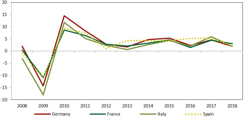 |
|
Source: Eurostat.
|
|
22
|
MINISTRY OF ECONOMY AND FINANCE
|
|
II. MACROECONOMIC FRAMEWORK
|
If we consider the data on foreign trade of goods, the sales growth
rates of Germany, Italy and Spain were equal to or just above 3 percent in 2018, halving in the first case and decelerating by about 5 percentage points for the other two
countries. Results in France, however, were more stable, with a 4 percent increase, down by just over half a percentage point. Like for the other EU partners, Italy’s change in
export values was largely supported by the EU zone (4.1 percent down from 7.2 percent in 2017) than by non-EU countries (1.7 down from 8.2 percent), the latter possibly affected by
lower price competitiveness.
As for total Italian exports to foreign markets, the United States
confirmed to be the most dynamic destination (5 percent), followed by Switzerland (8.7 percent). When it came to the EU zone, despite the slowdown, exports to major partners
continued to hold strong, with a 3.6 percent increase to Germany and 4.5 percent to France. Sales to Spain grew by more than 3 percent but slowed by over 7 percentage points; the
same goes for the UK (down to 1.1 from 2.3 percent in the previous year), reflecting the uncertainties surrounding Brexit. On the other hand, the contraction in exports to the main
emerging economies (Turkey, Russia and China) was quite significant, while, among the energy producing countries, the reduction in sales to the OPEC area has more than doubled
(-7.6 percent); Southern Common Market sales were also down, but to a lesser extent (by around 2 percent).
|
FIGURE II.6: PRICE COMPETITIVENESS INDEXES (January 2017 indexes = 100,
based on producer prices in manufacturing)
|
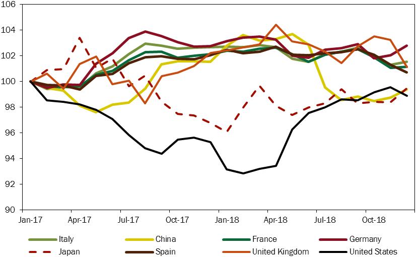
|
|
Source: Analysis based on Bank of Italy data.
|
|
MINISTRY OF ECONOMY AND FINANCE
|
23
|
|
ECONOMIC AND FINANCIAL DOCUMENT - SECT. I STABILITY PROGRAMME
|
|
FIGURE
II.7: EXPORTS OF ITALIAN GOODS TO MAJOR EU COUNTRIES
(January
2017 indexes = 100, seasonally adjusted data)
|
FIGURE II.8: EXPORTS OF ITALIAN GOODS TO MAJOR
NON-EU COUNTRIES
(January 2017 indexes = 100, seasonally adjusted data)
|
|
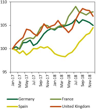
|
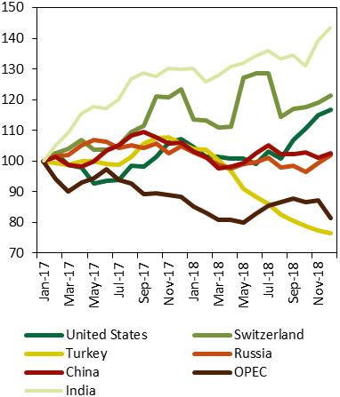
|
|
|
Source: Analysis based on ISTAT Coeweb data
|
||
Looking at sector performances, exports grew for all compared to
2017, although the pharmaceutical and transport sectors showed a more evident slowdown. Pharmaceutical sales increased by 4.7 percent (decelerating by over 10 percentage points),
with a more robust increase in the non-EU area (by over 7 percent), albeit with substantial reductions in exports to the United States (-6.5 percent), Turkey (-9.9 percent) and
Russia (-7 percent). In the European market, there was an increase in sales close to 3 percent, but with negative variations between 8 and 9 percent in exports to Belgium and the
United Kingdom.
In the transport sector, sales fell after five consecutive years of
expansion (-0.1 percent down from 7.2 percent in 2017), largely due to the contraction of the car sector (5.5 percent down from 11.5 percent in the previous year), especially
in non-European markets (-15.1 percent); the largest reductions were in the United States (-1.0 percent), Turkey (-28.4 percent) and China (-60.3 percent). Within the EU, this
sector grew by almost 3 percent. As for the other sectors, exports of chemicals, machinery and electrical appliances increased by around 3 percent, although the deceleration in
chemical exports was more than double (more than 6 percentage points) that of the other two sectors. Computer exports accelerated slightly (to 6.7 percent), while among the
traditional ‘Made in Italy’ sectors, textiles showed greater resilience (3.3 percent) compared to food, beverage and tobacco (2.5 percent).
Overall, Italy's trade balance (equal to about 39 billion, down
from 47.6 billion in 2017) remains among the highest in the European Union after Germany,
|
24
|
MINISTRY OF ECONOMY AND FINANCE
|
|
II. MACROECONOMIC FRAMEWORK
|
the Netherlands and Ireland13, despite it dropping to the lowest value in the past five years. The energy deficit rose to 42.6 billion, an increase of over 10 billion
compared to the previous year, due to higher imports and energy prices. The results in terms of current account balances remain positive (2.8 percent of GDP), substantially in
line with the previous two years.
|
F
O
C
U
S
|
Performance of Italian exports: obstacles and
the impact of external shocks
Among the various aspects relating to the performance of Italian exports, the recent
ISTAT Report14 indicates the factors that have most influenced export company activity
and the transmission of external shocks onto the various sectors. Turnover improved for 43 percent of Italian enterprises, thanks to higher investment and an increase
in employment, including of highly qualified personnel; however, the companies reporting a decrease rose to 22 percent (+2 pp). Manufacturing companies (about one
third) believe that foreign competition was the factor that worsened foreign turnover the most, while the pressure on prices by other Italian companies or bureaucratic
obstacles (including tariff barriers) are considered of little importance (12.4 and 11.1 percent respectively).
Sectoral competition among Italian businesses is a negative factor, especially when it
comes to non-metallic mineral products and leather goods; there is still pressure from foreign competitors in various sectors (oil and wood products, processing of
non-metallic minerals, metallurgy, metal products and machinery). About 40 and 20 percent of the companies in the automotive and metallurgy sectors report having
suffered from the ‘war of duties’.
Moving on to the effect of economic shocks on sector trends, the Social Network Analysis
of international interconnections allows us to determine to what extent the Italian foreign sector absorbs changes pertaining to the economic cycle or technological
progress. Investigations into the relationships of the Italian exporting sectors with Germany, the United States and China for the year 2014 reveal that four industry
sectors (machinery, chemicals, motor vehicles, metallurgy and metal products) have very close import/export ties with these three countries. Other sectors
(construction, non-metallic mineral products and health services) are shown to be significant for foreign sales in relation to their high degree of interconnection with
the markets considered; the service sector appears to be less important.
To summarise, the most advanced sectors of Italian industry and services have a greater
weight in connections with foreign countries than in domestic connections, with connections with Germany and the US being the most significant. For construction and
services (market and public), domestic inter-sectoral ties are predominant.
|
Looking at the short-term prospects, international downside risks
persist, linked to the uncertainty of the Sino-US trade relations, whose most recent developments could lead to a settlement. However, the dialogue between the United States
and the EU is still open, especially in the motor vehicle sector, which well represents their mutual commercial ties and within which Italy constitutes the third largest
exporter with 4.6 billion dollars in 2018, after Germany and the United Kingdom15. Further
opportunities could open up with the
___
13 Source: Eurostat, 15 February 2018.
14 ISTAT, ‘Report on the competitiveness of productive sectors’, 25 March 2019.
15 Source: ACEA (European Automobile Manufacturers’ Association), ‘EU-US automobile trade: facts and figures’, 18 March 2019.’
|
MINISTRY OF ECONOMY AND FINANCE
|
25
|
|
ECONOMIC AND FINANCIAL DOCUMENT - SECT.
I STABILITY PROGRAMME
|
recent initiatives involving China, in line with the negotiating rounds already
undertaken by the EU16.
Credit
trend
The positive trend of loans to the private sector continued
during 2018 and the most recent surveys confirm credit expansion even in early 2019. The preliminary data for the month of January released by the Bank of Italy show an
overall offer increase of 1 percent at unchanged legislation, driven by growing credit to households (2.6 percent y/y). However, there was a decrease in loans to
non-financial companies (-0.7 percent year on year), which interrupted the series of increases that began in late 2017.
Interest rates remained at limited and stable levels. At the
beginning of 2019, the harmonized rate applied to households for new mortgages was 2.3 percent, while that applied to consumer credit was 8.2 percent. Regarding new business
loans, the average rate under one million euro was just over 2 percent, while above this threshold the rate was equal to 1.04 percent.
|
FIGURE II.9: INTEREST RATES
FOR NON-FINANCIAL CORPORTATIONS AND HOUSEHOLDS (%)
|
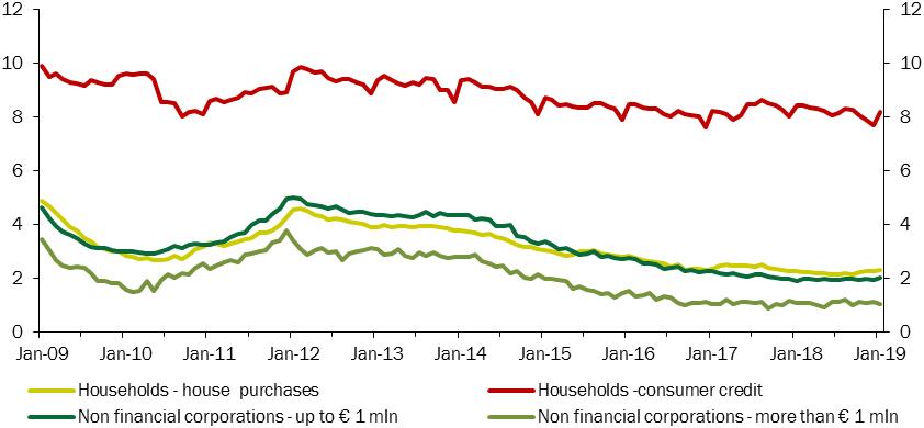
|
|
Note: The data refer to the harmonized rates applied to new loans
in euros.
Source: Bank of Italy.
|
Credit quality continues to improve, and there was a further
decrease in the incidence of impaired loans. Indeed, there was a sustained contraction in non-performing loans, marking a reduction of over 32 percentage points at unchanged
legislation in January. In particular, over the last year, impaired exposures with regard to non-financial companies fell slightly below 10 percent of total loans, (returning
to the values seen in late 2013), while household bad debts corresponded to around 4 percent of loans, comparable to 2011.
___
16 Source: European Commission, ‘Report of the 20th round of negotiations
for the EU-China Investment Agreement’, 1 March 2019 (http://trade.ec.europa.eu/doclib/docs/2019/march/tradoc_157772.pdf).
|
26
|
MINISTRY OF ECONOMY AND FINANCE
|
|
II. MACROECONOMIC
FRAMEWORK
|
|
FIGURE II.10: NON-PERFORMING LOANS TO RESIDENTS (as a
percentage of total loans)
|
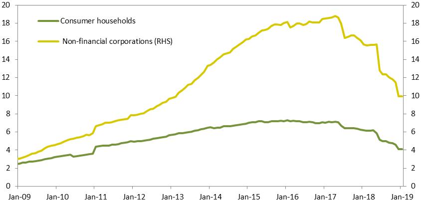 |
|
Source: Bank of Italy.
|
The most recent survey on bank credit in the euro zone (Bank
Lending Survey), published in January, shows a slight tightening of eligibility criteria for loans to Italian households and businesses. For the first quarter of the year,
intermediaries' expectations suggest substantially unchanged credit offer policies. The demand for business loans increased, mostly due to low interest rates and spending
connected to inventory and working capital. Similarly, the demand for mortgages by households is rising slightly thanks to low interest rates and still low house prices.
Prospects
for the Italian economy
Scenario under unchanged legislation
The most recent quantitative and qualitative
information confirms the continuation of a weak cyclical phase for the Italian economy, but with a slight improvement compared to the second half of 2018. The available
indices confirm a darker picture for the manufacturing sector and a more favourable and resilient picture for the services sector.
Confidence climate surveys of manufacturing
companies show a fall below average for the fourth quarter. Stocks of finished products also increased in the first quarter. The PMI remained below the expansion threshold
for six months. Industrial production increased beyond expectations in January (1.7 percent m/m) after the decline recorded in December; in terms of sectors, there was a
strong cyclical increase recorded in energy and non-durable consumer goods. Considering the most recent information, a flat industrial production trend is estimated for the
first quarter.
For the construction sector, the latest
production indications show weak cyclical increases. Positive signals come from the housing sector, still favoured by
|
MINISTRY OF ECONOMY AND FINANCE
|
27
|
|
ECONOMIC AND FINANCIAL DOCUMENT -
SECT. I STABILITY PROGRAMME
|
new mortgage rates; furthermore, confidence increased
significantly at the end of 1Q19, approaching record levels.
Turning to the services sector, the most
recent estimates point to a modest recovery in 1Q19 after the slight increase recorded in 4Q18; the available economic indices show a gradual increase in confidence. In
February, the PMI returned above the expansion threshold, 50.4, and in March it rose further to 53.1, confirming the ISTAT survey indications.
Consumer confidence surveys show a gradual
decline from the second half of 2018, reaching the lowest level since August 2017 in March 2019. In the first part of the year, consumers will enjoy greater purchasing
power thanks to a consumer price level still close to 1 percent (1.1 percent in March); however, core inflation, however, remains at 0.5 percent.
As for foreign demand, the available
indications show overall modest growth thanks to the stability of non-EU foreign trade recorded on an annual basis. Encouraging signs come from expectations of export
turnover improvements in the first quarter of 2019.
Growth for 2019 is revised downwards to 0.1
percent in real terms from the 1.0 percent estimated last December (see the box below, ‘Forecast errors for 2018 and revision of estimates for 2019 and the following
years’). It is estimated that the real growth rate will gradually progress in 2020, 2021 and 2022, and that GDP will grow by 0.6 percent in 2020, 0.7 percent in 2021 and
0.9 percent in 2022. Overall, the forecasts for 2019 and 2020 do not differ substantially from the average reported by Consensus Forecasts.
|
F
O
C
U
S
|
Forecast errors for 2018 and revision of
estimates for 2019 and the following years17
This is an in-depth analysis of the revision of growth forecasts formulated in the
Update to the Macroeconomic and Public Finance Framework published last December.
Firstly, we will analyse the deviations between the values forecast for 2018 and
the final figures published by ISTAT in March. These deviations are shown below in Table R1 (Column C, Forecast error).
Please bear in mind that the previous forecasts for 2018 were formulated in December and included the results of the third quarter and that the ISTAT data
published in March also include subsequent revisions; the differential reported in Column c is therefore attributable to both the fourth quarter forecast error
and the revision of the previous quarters.
As to the GDP, the forecasts were slightly higher than the final ISTAT figures,
mainly due to the 4Q18 performance, which was worse than expected. Based on the analysis of the aggregate demand components, which show worse than expected final
data on investments, the Italian economy was particularly penalized by the slowdown in the manufacturing sector globally and in particular in Germany. Italy’s
production of investment goods is closely linked to global demand and the supply chains in which Germany participates.
For 2019, it is possible to formulate indications on the scenario based on
unchanged legislation of the EFD (Italy’s Economic Planning Document) considering not only the data update but also the new assumptions on the international
macroeconomic scenario.
|
___
17 This box refers to the quarterly income statement data published on 5 March 2019 adjusted for working days. The annual raw data, not
adjusted for working days, of the 2018 GDP growth is 0.9 percent because there were 3 more working days. In 2019, the number of working days is the same as in 2018.
|
28
|
MINISTRY OF ECONOMY AND FINANCE
|
|
II. MACROECONOMIC
FRAMEWORK
|
|
TABLE R1: MACROECONOMIC
SCENARIO KEY VARIABLES (seasonally adjusted data)
|
||||||||||
|
|
2018
|
2019
|
||||||||
|
Forecasts and results
|
Factors accounting for
revision of the growth estimates (differences of growth rates)
|
Forecast
|
Delta – forecast and other
factors
|
|||||||
|
Update December 2018
|
Actual
|
Forecast
error
|
Delta -carry-over
effect |
Delta -international
scenario |
Update December 2018
|
DEF 2019
|
DEF –Update December 2018
|
Other
factors
|
||
|
a
|
b
|
c = b-a
|
d
|
e
|
f
|
g
|
h = g-f
|
i=h-d-e
|
||
|
GDP
|
0.9
|
0.8
|
-0.2
|
-0.2
|
-0.2
|
1.0
|
0.1
|
-0.81
|
-0.4
|
|
|
Imports of goods and services
|
1.9
|
1.8
|
-0.1
|
-0.3
|
-0.4
|
2.3
|
2.3
|
0.0
|
0.7
|
|
|
Household consumption
|
0.6
|
0.6
|
0.0
|
0.0
|
0.0
|
0.8
|
0.6
|
-0.2
|
-0.2
|
|
|
Gross fixed investment
|
4.0
|
3.2
|
-0.8
|
-0.4
|
0.1
|
2.5
|
0.7
|
-1.9
|
-1.5
|
|
|
Exports of goods and services
|
0.9
|
1.4
|
0.5
|
0.4
|
-1.0
|
2.4
|
2.1
|
-0.3
|
0.4
|
|
|
GDP deflator
|
1.1
|
0.8
|
-0.3
|
-0.2
|
0.0
|
1.4
|
0.9
|
-0.4
|
-0.2
|
|
|
Private Consumption deflator
|
1.1
|
1.1
|
0.0
|
0.0
|
0.2
|
1.4
|
1.0
|
-0.4
|
-0.6
|
|
Column D (Delta -carry-over effect) shows the difference of the statistical
carry-over effect of 2018 on 2019 between the value estimated in the last official update and the final value; in essence, this value shows how much the 2019
annual forecast would change due to the updating of the 2018 data with the same previous growth assumptions in each quarter of 2019. For the GDP, the carry-over
effect change is negative at -0.2 percentage points. The result below expectations of 4Q18 (-0.1 percent Q/Q) weighs on the carry-over effect. The carry-over on
the growth rate of the GDP deflator is also slightly negative, with repercussions on the nominal GDP estimate.
The revision of the international situation for December is explained in Column
E (Delta - International scenario), which shows the impact on the main variables estimated using the econometric model of the Treasury Department. The effect of
the new international framework is also negative and is affected by the significant downward revision of global demand gauged for Italy.
To summarise, the combined effect of the two variations explains half of the
downward GDP revision as shown in Column I (Other factors), which shows the difference between the actual forecast
revision (Column H = EFD-DBP) and the revision amount suggested by data analysis. The other half of the revision is linked to the still modest trend in GDP
expected for the first half of 2019, which is explained by an increased level of uncertainty and the slowdown in European manufacturing, especially in Germany,
still not fully considered by international exogenous variables.
Table R2 summarizes the impact on GDP growth of international developments,
comparing it with the assumptions made in the December 2018 Update.
Foreign demand dynamics gauged for Italy in the last quarter of 2018 resulted
weaker than those forecast in December and the estimates for 2019 were revised downwards from 3.9 percent to 2.3 percent. Consequently, the negative impact of
global demand on Italian exports and thus on GDP turns out to be greater in 2019, with a reduction in growth of 0.3 percent in 2019 and 0.1 percent in 2020.
However, for 2021, a 0.1 point growth increase is estimated.
|
|
MINISTRY OF ECONOMY AND FINANCE
|
29
|
|
ECONOMIC AND FINANCIAL DOCUMENT
- SECT. I STABILITY PROGRAMME
|
|
Late 2018 was characterized by a sudden fall of the oil prices ending in
December; while in early 2019, prices rose again. The current projections based on futures contracts foresee a modest reduction in oil price until 2022. In
contrast to December’s predictions, prices are slightly higher over the whole forecast horizon, especially in 2019 and 2020. This would lead to an impact of
-0.1 points on GDP in 2020.
On the exchange rates front, in 2018, there was a depreciation of the euro
against the dollar, which seems to be persisting into early 2019. For the currency forecast, we adopted a technical assumption that requires the exchange rate
to remain unchanged over time and equal to the average of the last 10 working days. The update of the effective nominal exchange rate compared to December
shows a 0.6 percent greater depreciation of the euro compared to other currencies in 2019. The macroeconomic impact is up by 0.1 percentage points on GDP
growth in 2019 and 2020.
The profile of the interest rates on government bonds proves most
accommodating for the economy in the three-year period 2019-2021. Furthermore, a reduction is foreseen in the differential between BTP and ten-year BUND and
improved credit conditions. According to econometric model estimates, these effects would bring a growth benefit of 0.2 points in 2020 and 0.3 points in 2021.
Altogether, the new international setting is less favourable with respect to
the December update in 2019, due to the slowdown in global demand, only partially offset by the benefits deriving from euro depreciation. According to
econometric model estimates, the economy will benefit from 0.4 points growth in 2021 due to the more favourable interest rates.
|
|
TABLE R2: ESTIMATED
EFFECT OF CHANGES IN INTERNATIONAL EXOGENOUS VARIABLES (IMPACT ON GROWTH RATES)
|
|||||
|
2018
|
2019
|
2020
|
2021
|
||
|
1. World trade
|
0.0
|
-0.3
|
-0.1
|
0.1
|
|
|
2. Nominal effective exchange rate
|
0.0
|
0.1
|
0.1
|
0.0
|
|
|
3. Oil price
|
0.0
|
0.0
|
-0.1
|
0.0
|
|
|
4. Interest rate assumptions
|
0.0
|
0.0
|
0.2
|
0.3
|
|
| |
Risk (or sensitivity) analysis of exogenous variables
|
|
The international scenario envisaged in terms of general macroeconomic trends
contributes decisively to the evolution of the Italian economy, notoriously open towards foreign trade. World trade dynamics, exchange rates, oil prices and
financial market conditions outline the international scenario and the profile of these variables reflects standard projection methods employed at major
national and international forecasting centres. Since these variables appear to have uncertain trends, it seems appropriate to provide an assessment of some
of the risks inherent in the overview at unchanged legislation. Using the ITEM econometric model, we simulated some alternative scenarios with main
international exogenous variables different from those foreseen in the overview based on unchanged legislation, in order to assess possible impacts on the
growth of the Italian economy. We designed four alternative scenarios, each focusing on a specific element of (positive and negative) risk for the national
economy. The first three simulations refer to exogenous variables of the international framework: global demand, nominal effective exchange rate for Italy and
oil price.
The second half of 2018 was characterized by the gradual slowdown in world trade leading to a downward revision of its growth prospects for 2019. For the
current year, the predicted growth rate of global demand for Italy is 2.3 percent lower than both in 2018 and envisaged for this year in the last EFD
Update. In this context, the dynamics of global demand accelerates in 2020 (3.9 percent) and stabilizes in the following two years (3.8 and 3.7 percent,
respectively). However, uncertainty about the growth prospects of some emerging economies leads us to consider a further unfavourable scenario in which the
global demand
|
|
30
|
MINISTRY OF ECONOMY AND FINANCE
|
|
II. MACROECONOMIC
FRAMEWORK
|
|
growth rate gauged for Italy is 0.3 points lower than the baseline scenario in 2019 and one percentage point lower in the following three years18. With regard to the trend in exchange rates, the framework at unchanged
legislation adopts the technical assumption of constant exchange rates over the forecast horizon19; the alternative scenario, on the other hand, uses bilateral forward exchange rates with different contractual maturities
until 2022. This approach gives rise to a lower depreciation of the nominal effective exchange rate in 2019 compared to the baseline scenario (by 0.7 and 0.4
percent, respectively). In the following three years there is instead an overall 3.2 percent appreciation of the euro (understood as a change in the nominal
effective exchange rate) as opposed to the lack of change predicted in the scenario based on unchanged legislation.
The third risk scenario concerns oil prices. The scenario at unchanged
legislation is based on the price of crude oil futures contracts and foresees a gradual reduction in oil price from $64.8 a barrel in 2019 to $61.7 in 2022.
The alternative scenario assumes crude oil prices that are $10 higher than the reference scenario, starting in the second quarter of 2019 (for example, a $72
per barrel oil price is assumed for 2019).
Lastly, with regard to the financial conditions of the economy, a more
favourable scenario is considered compared to the scenario at unchanged legislation. A scenario of greater saver and financial operator confidence is assumed
in which, from the second quarter of 2019, the rate of return on ten-year BTPs is 100 basis points lower than the corresponding baseline scenario. Therefore,
in this scenario, the lower BTP-BUND spread would affect the interest rates charged by banks, making the terms of loans to private individuals more
favourable.
The results of the risk sensitivity analysis of the macroeconomic scenario at
unchanged legislation are shown in Table R1. Reduced growth in global demand weakens Italian export dynamics and leads to a fall in product growth in the
four-year period 2019-2022. In 2022, GDP stands at around 0.7 percentage points lower than the corresponding baseline scenario. The appreciation of the euro
(in particular the nominal effective exchange rate for the Italian economy) and the increase in oil prices may also slow growth in the coming years. In terms
of financial conditions, the assumption of a more favourable scenario associated with lower risk premiums demanded by investors has favourable effects on GDP
as well as on consumption and investment.
In conclusion, due to the uncertainty of the international scenario, three
risk scenarios were assumed that weaken the growth of the Italian economy through less lively foreign demand or a less favourable trend in exchange rates and
crude oil prices. On the other hand, improved financial conditions would generate benefits that would be transferred primarily to domestic demand.
|
|
TABLE R1:
IMPACT OF RISK SCENARIOS ON GDP (impact on growth rates)
|
|||||
|
2019
|
2020
|
2021
|
2022
|
||
|
World trade
|
-0.1
|
-0.2
|
-0.2
|
-0.2
|
|
|
Nominal effective exchange rate
|
0.0
|
-0.2
|
-0.4
|
-0.3
|
|
|
Oil price
|
-0.1
|
-0.3
|
-0.1
|
0.0
|
|
|
More favourable financial conditions
|
0.0
|
0.3
|
0.4
|
0.4
|
|
The downward revision also takes into account the
assessment of medium-term geopolitical risks. In the final year of the forecast, GDP growth is estimated at less than 1 percent; the greater degree of forecast
uncertainty, connected to a
___
18 The new global demand gauged for Italy is the result of a 0.25 percent reduction in growth compared to the previous quarter, starting
from the second quarter of 2019.
19 We consider the average of the most recent daily quotations, recorded in the last ten working days.
|
MINISTRY OF ECONOMY AND FINANCE
|
31
|
|
ECONOMIC AND FINANCIAL
DOCUMENT - SECT. I STABILITY
PROGRAMME
|
longer time horizon, makes it appropriate to adopt a technical approach
based on which the trend in economic growth converges towards that of the potential product. During the entire forecast period, the main driver of growth is
domestic demand, while foreign demand provides a marginally positive contribution only at the end of the period.
In the scenario based on unchanged legislation,
starting from the end of the second quarter of 2019, household consumption spending will be sustained by the entry into force of the two measures of Law 26/2019, Reddito di Cittadinanza (Citizen’s Income) and early retirement (so-called ‘Quota 100’) thanks to the generational turnover of
those in employment. The effect of these measures on GDP and the main components is described in the two boxes below.
On the other hand, in 2020-2021, the positive effect
of the two measures is in part reduced by the VAT increase under the 2019 Budget Law. Although it is not assumed that the hike in VAT will be fully transferred to
product prices, any increase in consumer prices affects real disposable income and the propensity to consume; the savings rate falls slightly to just over 8 percent
at the end of the period.
With a gradual slowdown from the second half of 2018,
investments are expected to increase only slightly in 2019 and then return to modest expansion in subsequent years.
For the current year, weak investment in machinery is
affected by the uncertain global context, in particular due to the ongoing commercial tensions between the USA and China, though it may also be influenced by less
favourable credit conditions. In January, data on business loans fell below zero; in addition, bank credit surveys revealed a slight contraction in loans to
businesses. From 2020, there is the positive impact of the recovery in exports.
Investment in construction grows at a moderate rate
thanks to real estate being favoured by accommodative monetary policies and renovation incentives.
Exports increase on average at a rate lower than that
of the foreign markets relevant to Italy due to the uncertainty generated by commercial tensions. Imports also experience moderate growth, in line with domestic
demand. The current account balance stands at 2.5 percentage points of GDP at the end of the period.
Labour market dynamics are influenced by the weak
cyclical phase and the effects of Law 26 of 28 March 2019 on Citizen’s Income and Quota 100. Workforce employment numbers decrease by 0.3 percent and then return
above zero with growth of 0.6 percent at the end of the period. In 2019, hours worked per employee continue to increase, as only a partial replacement of Quota 100
retirees is initially assumed. Both Citizen’s Income and Quota 100 have an impact on labour supply; the former will lead to a bigger workforce and the latter will
do the opposite. Taking into account the assumptions adopted for the simulations and the weak cyclical phase, the unemployment rate is expected to increase slightly
in 2019 (11.0 percent) and in 2020 (11.2 percent) and then decrease gradually, returning to the 2018 levels at the end of the period. Per capita wage dynamics will
slow down in 2019 compared to 2018 and remain modest in the following three years. The growth rate of unit labour costs, influenced by the moderate growth in
productivity, will increase on average by 1 percent over the forecast horizon (2019-2022).
|
32
|
MINISTRY OF ECONOMY AND FINANCE
|
|
II. MACROECONOMIC FRAMEWORK
|
Inflation will remain contained in 2019 (1.0
percent) due to the fall in energy prices and the slowdown in domestic demand. In 2020 and 2021, price growth will be affected by the VAT increase.
|
F
O
C
U
S
|
An assessment of the
macroeconomic impact of the Citizen’s Income measures
The purpose of this box is to evaluate the macroeconomic effects of the
Government’s actions concerning citizen’s income and pension adopted by Decree Law 4 of 28 January 2019, later amended and converted into Law 26 of 28
March 2019. Citizen’s Income is an income support scheme for poor households accompanied by measures to encourage beneficiaries to engage in the labour
market and find employment.
The provision defines the intended beneficiaries of the benefit, the
financial eligibility requirements and the total annual sum provided, which depends on the household, income and home ownership status. In 2019, the
Budget Law allocated 7.1 billion of public funding to the scheme, of which 5.6 billion for Citizen’s Income and 274 million for the continuation of the
Inclusion Income. The remaining amount was considered higher expenditure for improving job centres and active labour market policies. In 2020 and 2021,
the overall allocations amount to 8.1 and 8.3 billion, of which 7.2 and 7.4 billion for benefit disbursement and the rest for job centres and active
employment policies. A total cost of 8.3 billion has been forecast for 2022 and the years following.
According to ISTAT estimates, the recipients of citizen’s income and
pension could reach 2.706 million, of which 1.791 million of working age (16-64); of these, 57 percent are either employed or seeking employment. Because
eligibility for Citizen’s Income is subject to actively seeking work, this measure should immediately increase participation in the labour market through
recourse to job centres by persons previously not seeking employment. ISTAT has estimated that the national workforce will increase by 470,000 thanks to
this Government action.
The macroeconomic impact of the Citizen’s Income was evaluated using the
ITEM econometric model. The simulation was drawn as follows: the payment of citizen’s income and pension is assimilated to a current transfer to
households assuming that they will increase compared to the baseline scenario from the second quarter of 2019. The costs of improving job centres are
classified as higher public spending to increase the number of centre operators. In line with the ISTAT estimate, we also assume an exogenous increase in
workforce compared to the baseline scenario from the second quarter of 2019, reaching 470,000 units in the second quarter of 2020 and remaining at this
level in the years following. This increase occurs gradually, also due to the technical characteristics of the ISTAT sample survey, which form the basis
of the statistical employment and unemployment data considered in the macroeconomic forecast.
The assessment involved certain additional assumptions. Firstly, the
assumption of a marginal propensity to consume in relation to disposable income of 0.8, from the very beginning. This level coincides with that implicit
in the model, although in the model it is reached more gradually over time. This decision takes into account the evidence that less well-off individuals,
for whom the measure was put in place, have a higher than average propensity to consume, including in the short term, and the fact that ITEM, as an
aggregate model, is unable to illustrate the variations in behaviour according to individual income. Furthermore, the provision envisages penalties in the
event that the monthly payment of the financial benefit does not result in consumption expenditure for the same month. On the other hand, a 0.8 propensity
to consume is consistent with the hypothesis that some beneficiaries may increase their propensity to save on incomes other than the Citizen’s Income.
Another aspect concerns the trend in average wages and employment. In
general, an exogenous increase in labour market participation should lead to an increase in
|
|
MINISTRY OF ECONOMY AND FINANCE
|
33
|
|
ECONOMIC AND
FINANCIAL DOCUMENT - SECT. I STABILITY PROGRAMME
|
|
unemployment and, consequently, wage deflation. Both the increase in
labour supply compared to the baseline scenario and the lower bargaining power of workers due to higher unemployment contribute to this effect in the
model. However, in the simulation of the model, it was assumed that salaries would remain unchanged with respect to the baseline scenario for the first
two years of the simulation horizon, given that the exogenous increase in labour supply associated with enrolment at job centres is initially purely
statistical and will become reality over time. On the contrary, starting from the third year (2021), salaries are allowed to vary endogenously in the
model; these tend to decrease compared to the baseline scenario, in part because the entry level wages for new employees are often lower than the
national average salary. This occurs despite the fact that the provision established a minimum wage (858 euro) to be used as a benchmark for assessing
offers of work, against which refusal to accept a job leads to loss of Citizen’s Income.
Furthermore, it is reasonable to assume that strengthening job centres
may partly improve the functioning of the labour market, with a positive impact on employment from the third year, in addition to that of the first year
pertaining to the greater aggregate demand triggered by the scheme. An increase in the demand for work tends to reabsorb in part the unemployment rate
compared to the baseline scenario and goes hand in hand with lower salary levels. It is hoped that the effect of active employment policies, such as
higher training, together with the effect of the minimum wage defined in the provision as a benchmark for an appropriate job offer, will lift wages
above the baseline scenario in the medium to long term. This would reduce the population eligible for the Citizen’s Income, insofar as more low-income
workers would earn salaries above the income support threshold.
The macroeconomic impact of the Citizen’s Income is shown in Table R1.
The percentage variation in GDP increases by 0.2 percentage points compared to the baseline scenario in 2019 and in 2020 and by 0.1 percentage points in
2021. After four years, in 2022, the level of the product is 0.5 percentage points higher than that of the baseline scenario. Considering that the
overall costs of public funding of the measure ex ante is around 0.4 percentage points of GDP each year, the results recorded in Table R1 reflect an
implicit multiplier on the product of 0.6 in the first year, 1 in the second and 1.1 in the third.
|
|
TABLE
R1: ASSESSMENT OF THE MACROECONOMIC IMPACT OF CITIZEN’S INCOME (differences in percentage variation rates compared to the baseline scenario)
|
|||||
|
|
2019
|
2020
|
2021
|
2022
|
|
|
GDP
|
0.2
|
0.2
|
0.1
|
0.0
|
|
|
GDP deflator
|
0.1
|
0.0
|
0.0
|
0.0
|
|
|
Consumption deflator
|
0.0
|
0.0
|
0.1
|
0.0
|
|
|
Consumption
|
0.5
|
0.2
|
0.1
|
0.1
|
|
|
Investment
|
0.1
|
0.4
|
0.0
|
0.0
|
|
|
Exports
|
0.0
|
0.0
|
0.0
|
0.0
|
|
|
Imports
|
0.1
|
0.4
|
0.0
|
0.2
|
|
|
Employment
|
0.1
|
0.2
|
0.4
|
0.4
|
|
|
Participation rate (*)
|
0.4
|
1.2
|
1.3
|
1.5
|
|
|
Unemployment rate (*)
|
0.4
|
1.3
|
1.2
|
0.9
|
|
|
(*) Difference compared to the baseline scenario
|
|||||
|
The expansive effect on economic activity is determined by consumption
deriving from higher disposable income due to the income support scheme and greater employment. In
|
|
34
|
MINISTRY OF ECONOMY AND FINANCE
|
|
II. MACROECONOMIC FRAMEWORK
|
|
2022, employment is up by 1.1 percentage points compared to the baseline
scenario, with an increase of 260,000 in work20. The unemployment rate
increases, reaching a 1.3 percentage points higher than the baseline scenario in 2020. This gap gradually narrows n the following years.
|
|
F
O
C
U
S |
An assessment of the
macroeconomic effects of pension measures
Legislative Decree 4 of 28 January 2019, converted with amendments into
Law 26 of 28 March 2019, includes several retirement pension measures in addition to the Citizen’s Income. The principal regulatory amendment concerns
the new access channel to pensions, introducing the joint requirement of at least 38 years of pension contributions and being at least 62 years of age
(known as ‘Quota 100’). The possibility of early retirement through the ‘Quota 100’ mechanism is only granted to those who meet the requirements between
2019 and 2021. Furthermore, the years of contributions for early retirement is reduced by five months, bringing it to 42 years and 10 months for men and
41 years and 10 months for women. It is also established that these requisites shall not be adjusted for life expectancy increases until 202621. The decree technical report, based on estimates of the early
retirement take-up rate, predicts the greatest number of retirement benefits at the end of each year in relation to the provision, together with the
corresponding annual cost for public finance. In particular, the greatest number of pensions associated with the provision is estimated at 290,000 at
the end of 2019, 327,000 at the end of 2020 and 356,000 and 296,000 at the end of 2021 and 2022. In the first four years, the greatest expense would
amount to 3.8 billion in 2019. 7.9 billion in 2020, 8.4 billion in 2021 and 7.9 billion in 2022. For private employees who benefit from retirement under
the new requirements, early severance indemnity devolved to the INPS management fund must also be considered. The effects of this aspect for public
finance constitute costs of 585 million in 2019, while they are lower in 2020 and 2021; for the following years, the effects are of savings instead.
This box shows the results of the assessment of the macroeconomic impact
of the measure, performed using the ITEM econometric model. The increase in number of pensions was distributed according to type of worker according to
the estimates of the technical report, which distinguishes at the end of each year early retirement figures for employees in the private sector,
self-employed workers and state employees. These methods thus included the exogenous decrease in employment for each of the three sectors.
All other conditions being equal, the contraction in the
number of persons in employment following the new retirement scheme would leads to a corresponding reduction in the workforce. A similar decrease in
both employment and workforce would push the unemployment rate above the baseline scenario. However, the generational turnover, i.e. the replacement
of workers who opted for ‘Quota 100’ with new recruits, pushes in the
|
___
20 This increase could be considered too optimistic if we take into account the recent empirical evidence on the impact of job
vacancies on numbers in employment (vacancy rate) in Italy. This impact is around 1.2 percentage points, only slightly below the expected percentage increase in
employment in the fourth year of the simulation horizon (1.1 percent). It is noted, however, that the other measure included in the decree currently being
converted into law, on pensions, called ‘Quota 100’, could cause, by its nature, a significant increase in vacancy rate in conjunction with individual
pre-retirement decisions.
21 With respect to the maturity date of the requisite, Law 26/2019 provides for a three-month window for private sector workers
to access retirement with the first effective date on 1 April 2019. For public sector employees, the window is six months with the first effective date on 1
August 2019 (1 September for workers in the school sector only). The law includes various other measures that affect pension spending. Among these, the women’s
option, the extension of the social EPA and the suspension to 2026 of the adjustment to the increase in life expectancy of the pension requirements for
early-starting workers. Assessment of the macroeconomic impact of pension measures also considered these measures.
|
MINISTRY OF ECONOMY AND FINANCE
|
35
|
|
ECONOMIC AND
FINANCIAL DOCUMENT - SECT. I STABILITY PROGRAMME
|
|
opposite direction. If we assume that the new recruits come entirely
from among the unemployed, a replacement rate of 10 percent would be enough to guarantee the unemployment rate stays the same. Therefore, if, as is
plausible, the generational turnover is above 10 percent, the unemployment rate will drop with other conditions being equal.
The results are shown in Table R1. The percentage variation in GDP
remains unchanged in 2019 compared to the baseline scenario, increases by 0.1 percentage points both in 2020 and 2021 and remains unchanged in 2022.
After four years, in 2022, the product level therefore increases by 0.2 percentage points compared to the baseline scenario. The 2019 GDP trend is
negatively affected by the decrease in public sector value added, measured based on employee numbers in the general government sector.
|
|
TABLE
R1: ASSESSMENT OF THE MACROECONOMIC IMPACT OF SOCIAL SECURITY MEASURES (differences in percentage variation compared to the baseline scenario)
|
|||||
|
2019
|
2020
|
2021
|
2022
|
||
|
GDP
|
0.0
|
0.1
|
0.1
|
0.0
|
|
|
GDP deflator
|
-0.1
|
0.0
|
0.1
|
0.2
|
|
|
Consumption deflator
|
-0.1
|
-0.1
|
0.1
|
0.2
|
|
|
Consumption
|
0.1
|
0.2
|
0.2
|
0.0
|
|
|
Employment
|
-0.3
|
-0.2
|
0.1
|
0.1
|
|
|
Participation rate (*)
|
-0.1
|
-0.3
|
-0.3
|
-0.3
|
|
|
Unemployment rate (*)
|
-0.2
|
-0.6
|
-0.8
|
-0.9
|
|
|
(*) Difference compared to the baseline scenario.
|
|||||
|
The employment trend in the second half of 2019 is affected by the
exit from the labour market of subscribers to the scheme and their partial replacement by new recruits. The replacement rate is estimated by the ITEM
model at around 35 percent. In subsequent years, the percentage replacement estimated by the model stands at between 70 and 80 percent of early
retirement22. The gradual reduction in unemployment compared to the
baseline scenario, reaches 0.9 percentage points in the fourth year (2022). This, together with the fact that lower unemployment generates a slight
upward pressure on wages, has a positive effect on private consumption, which, after three years, is 0.5 percentage points greater than the baseline
scenario.
The results obtained show an increase in labour productivity compared
to the baseline scenario, which reaches 0.5 percentage points in the third year. This increase can be attributed to a greater intensity of use of the
labour factor, especially at the beginning of the simulation period. Subsequently, the gradual introduction of new recruits to the production process
brings productivity back down to baseline scenario levels. The effects on the average salary are initially negative (due to the change in composition
of employees), whereas they become positive later on. This is also reflected in the variation in GDP deflator, slightly lower than the baseline
scenario in the first year, zero in the second and positive in 2021 and 2022.
|
___
22 The effects of the measure to introduce the Citizen’s Income and the reform of job centres, included under Law
26/2019, should generate an increase in employment opportunities, thus helping to fill positions left vacant by early retirement.
|
36
|
MINISTRY OF ECONOMY AND FINANCE
|
|
II. MACROECONOMIC FRAMEWORK
|
|
TABLE II.1: MACROECONOMIC SCENARIO based on
unchanged legislation (percentage variations, unless otherwise indicated) (1)
|
|||||
|
2018
|
2019
|
2020
|
2021
|
2022
|
|
|
INTERNATIONAI EXOGENEOUS
VARIABLES
|
|||||
|
World Trade
|
3.8
|
2.5
|
3.7
|
3.8
|
3.9
|
|
Oil Price (Brent, USD/barrel, futures)
|
71.3
|
64.8
|
64.6
|
62.9
|
61.7
|
|
USD/EUR exchange rate
|
1.181
|
1.135
|
1.134
|
1.134
|
1.134
|
|
ITALY MACRO DATA (VOLUMES)
|
|||||
|
GDP
|
0.9
|
0.1
|
0.6
|
0.7
|
0.9
|
|
Imports
|
2.3
|
2.2
|
2.5
|
2.5
|
2.5
|
|
Domestic final consumption
|
0.5
|
0.4
|
0.6
|
0.6
|
0.6
|
|
Household consumption and NPISH
|
0.6
|
0.6
|
0.6
|
0.7
|
0.8
|
|
Government expenditure
|
0.2
|
-0.3
|
0.4
|
0.1
|
0.0
|
|
Investment
|
3.4
|
0.7
|
1.2
|
1.3
|
1.5
|
|
- machinery, equipment and
intangible assets
|
2.1
|
0.1
|
1.1
|
1.3
|
1.6
|
|
- transportation means
|
14.5
|
-1.4
|
1.3
|
1.4
|
1.4
|
|
- construction
|
2.6
|
1.4
|
1.3
|
1.3
|
1.4
|
|
Exports
|
1.9
|
2.1
|
2.3
|
2.5
|
2.6
|
|
Memo item: Current account balance (% of GDP)
|
2.6
|
2.6
|
2.5
|
2.5
|
2.5
|
|
CONTRIBUTIONS TO GDP GROWTH (1)
|
|||||
|
Net exports
|
-0.1
|
0.0
|
0.0
|
0.0
|
0.1
|
|
Inventories
|
0.0
|
-0.2
|
0.0
|
0.0
|
0.0
|
|
Domestic demand net of inventories
|
1.0
|
0.4
|
0.7
|
0.7
|
0.8
|
|
PRICES
|
|||||
|
Imports deflator
|
2.9
|
1.7
|
1.8
|
1.7
|
1.6
|
|
Exports deflator
|
1.7
|
1.4
|
1.7
|
1.6
|
1.6
|
|
GDP deflator
|
0.8
|
1.0
|
1.9
|
1.7
|
1.5
|
|
Nominal GDP
|
1.7
|
1.2
|
2.6
|
2.5
|
2.4
|
|
Consumption deflator
|
1.1
|
1.0
|
2.3
|
1.8
|
1.5
|
|
LABOUR
|
|||||
|
Cost of Labour
|
2.0
|
1.2
|
1.3
|
1.2
|
1.6
|
|
Productivity (measured on GDP)
|
0.1
|
0.3
|
0.4
|
0.3
|
0.3
|
|
ULC (measured on GDP)
|
1.9
|
0.9
|
0.9
|
1.0
|
1.3
|
|
Employment (FTEs)
|
0.8
|
-0.2
|
0.2
|
0.5
|
0.6
|
|
Unemployment rate
|
10.6
|
11.0
|
11.2
|
10.9
|
10.6
|
|
Employment rate (age 15-64)
|
58.5
|
58.7
|
58.9
|
59.3
|
59.8
|
|
Memo item: Nominal GDP
(absolute values in millions of euro)
|
1,756,982
|
1,777,899
|
1,823,329
|
1,868,945
|
1,914,457
|
|
(1) Discrepancies, if any, are
due to rounding.
|
|||||
|
(2) Source: ISTAT.
|
|||||
|
Note: The macroeconomic
scenario relating to international exogenous variables was developed based on the information available as at 9 April 2019.
|
|||||
|
GDP and components by volume
(chained values in reference year 2010), data not adjusted for business days.
|
|||||
Policy scenario
As described in chapter 1, the policy scenario
includes the effects on the Italian economy of the two legislative decrees presented at the same time as the Stability Plan, including measures to stimulate
private investment and local government investment (‘Growth’ Leg. D.) and measures to streamline public work approval procedures (‘Unlock Sites’ Leg. D.).
The policy scenario confirms current tax legislation pending the definition of alternative measures in the
|
MINISTRY OF ECONOMY AND FINANCE
|
37
|
|
ECONOMIC AND
FINANCIAL DOCUMENT - SECT. I STABILITY PROGRAMME
|
upcoming months, in preparation of the 2020 Budget Law. Greater
public investment is also predicted, especially for 2020 and 2021.
|
TABLE II.2: BASE ASSUMPTIONS
|
|||||
|
|
2018
|
2019
|
2020
|
2021
|
2022
|
|
Short-term interest rate (1)
|
n.a.
|
-0.01
|
0.85
|
1.75
|
2.39
|
|
Long-term interest rate
|
2.54
|
2.73
|
3.13
|
3.49
|
3.77
|
|
USD/EUR exchange rates
|
1.181
|
1.135
|
1.134
|
1.134
|
1.134
|
|
Change in the nominal effective exchange rate
|
2.8
|
-0.7
|
0.0
|
0.0
|
0.0
|
|
World GDP, excluding EU
|
3.9
|
3.3
|
3.5
|
3.6
|
3.6
|
|
EU GDP
|
1.9
|
1.5
|
1.7
|
1.6
|
1.6
|
|
Global demand weighted for Italy
|
3.9
|
2.3
|
3.9
|
3.8
|
3.7
|
|
World imports volumes, , excluding EU
|
3.9
|
2.4
|
4.0
|
4.1
|
4.1
|
|
Oil price (Brent, USD/barrel)
|
71.3
|
64.8
|
64.6
|
62.9
|
61.7
|
|
(1) Short-term interest rate is understood to
mean the average of the rates applied to 3-month government bonds issued during the year. Long-term interest rate is understood to mean the
average of the rates applied to 10-year government bonds issued during the year.
|
|||||
|
TABLE
II.3a: MACROECONOMIC PROSPECTS
|
||||||
|
|
2018
|
2018
|
2019
|
2020
|
2021
|
2022
|
|
Level (1)
|
% Variations
|
|||||
|
Real GDP
|
1,614,865
|
0.9
|
0.2
|
0.8
|
0.8
|
0.8
|
|
Nominal GDP
|
1,756,982
|
1.7
|
1.2
|
2.8
|
2.6
|
2.3
|
|
REAL GDP COMPONENTS
|
||||||
|
Private consumption (2)
|
969,098
|
0.6
|
0.6
|
0.7
|
0.7
|
0.6
|
|
Public spending (3)
|
314,173
|
0.2
|
-0.4
|
0.8
|
0.1
|
-0.1
|
|
Gross fixed investment
|
296,078
|
3.4
|
1.4
|
2.0
|
1.8
|
1.6
|
|
Inventories (% of GDP)
|
0.0
|
-0.2
|
0.0
|
0.0
|
0.0
|
|
|
Exports of goods and services
|
517,576
|
1.9
|
2.1
|
2.3
|
2.4
|
2.6
|
|
Imports of goods and services
|
484,721
|
2.3
|
2.2
|
2.7
|
2.6
|
2.5
|
|
CONTRIBUTIONS TO REAL GDP GROWTH
|
||||||
|
Domestic demand
|
-
|
1.0
|
0.5
|
0.9
|
0.8
|
0.7
|
|
Change in inventories
|
-
|
0.0
|
-0.2
|
0.0
|
0.0
|
0.0
|
|
Net exports
|
-
|
-0.1
|
0.0
|
-0.1
|
0.0
|
0.1
|
|
(1) Millions.
|
||||||
|
(2) Final consumption spending of households and
non-profit private social institutions serving households (I.S.P.).
|
||||||
|
(3) Public administrations.
|
||||||
|
Note: Discrepancies, if any, are due to
rounding.
|
||||||
The effects of the above measures on the
economy will result in additional GDP growth of 0.1 percentage points in 2019, 0.2 percentage points in 2020 and 0.1 percentage points in 2021. On the
other hand, in the last year of the forecast, 2022, GDP growth is 0.1 percentage points lower than the figure at unchanged legislation, due to a more
challenging deficit target and measures to reduce public expenditure and combat tax evasion.
Therefore, real GDP growth will be 0.2
percent in 2019 and 0.8 percent in the three years after that. Compared to the macroeconomic overview based on unchanged legislation, the greater growth
in 2019-2021 comes essentially from the gross fixed investment component.
|
38
|
MINISTRY OF ECONOMY AND FINANCE
|
|
II. MACROECONOMIC FRAMEWORK
|
|
TABLE II.3b: PRICES
|
||||||
|
2018
|
2018
|
2019
|
2020
|
2021
|
2022
|
|
|
Level
|
||||||
|
GDP deflator
|
108.8
|
0.8
|
1.0
|
2.0
|
1.8
|
1.6
|
|
Private consumption deflator
|
110.1
|
1.1
|
1.0
|
2.3
|
1.9
|
1.6
|
|
HICP
|
102.5
|
1.1
|
1.0
|
2.3
|
1.9
|
1.6
|
|
Public consumption deflator
|
105.3
|
2.1
|
0.7
|
1.2
|
0.0
|
0.4
|
|
Investment deflator
|
106.6
|
0.5
|
0.6
|
1.6
|
1.9
|
1.7
|
|
Export deflator
|
107.8
|
1.7
|
1.4
|
1.7
|
1.7
|
1.6
|
|
Import deflator
|
106.0
|
2.9
|
1.7
|
1.8
|
1.7
|
1.5
|
|
TABLE II.3c: LABOUR MARKET
|
||||||
|
2018
|
2018
|
2019
|
2020
|
2021
|
2022
|
|
|
Level
|
||||||
|
Employment (national accounts)
|
25,335
|
0.9
|
-0.3
|
0.2
|
0.7
|
0.6
|
|
Total hours worked
|
43,641,891
|
1.1
|
-0.2
|
0.3
|
0.7
|
0.6
|
|
Unemployment rate
|
10.6
|
11.0
|
11.1
|
10.7
|
10.4
|
|
|
Labour productivity measured on the employment
|
63,739
|
0.0
|
0.6
|
0.6
|
0.0
|
0.0
|
|
Labour productivity measured on hours worked
|
37.0
|
-0.2
|
0.4
|
0.5
|
0.1
|
0.1
|
|
Compensation of employees
|
706,934
|
3.3
|
1.3
|
1.8
|
1.9
|
2.2
|
|
Compensation per employee
|
41,265
|
2.0
|
1.2
|
1.5
|
1.3
|
1.6
|
|
(1) Units of measurement: thousands of units for
employed in national accounts and total hours worked; euro at constant values for labour productivity; millions of euro at current values for
income from employment and euro for labour costs.
|
||||||
|
TABLE II.3D: SECTORAL ACCOUNTS
|
|||||
|
% of GDP
|
2018
|
2019
|
2020
|
2021
|
2022
|
|
Net lending/borrowing with the rest of the world
|
2.3
|
2.3
|
2.2
|
2.1
|
2.1
|
|
Balance of goods and services
|
2.5
|
2.5
|
2.3
|
2.3
|
2.4
|
|
Balance of primary income and transfers
|
-0.1
|
-0.1
|
-0.1
|
-0.1
|
-0.2
|
|
Capital account
|
-0.1
|
-0.1
|
-0.1
|
-0.1
|
-0.1
|
|
Borrowing/surplus of the private sector
|
4.5
|
4.7
|
4.3
|
4.0
|
3.6
|
|
Borrowing/surplus of the public administrations
|
-2.1
|
-2.4
|
-2.1
|
-1.8
|
-1.5
|
|
MINISTRY OF ECONOMY AND FINANCE
|
39
|
III. NET BORROWING AND PUBLIC DEBT
III.1 FINAL
DATA AND FORECASTS AT UNCHANGED LEGISLATION
According to the provisional estimates
published by ISTAT on 9 April, the ratio of general government net borrowing to GDP is at 2.1 percent in 2018, with an improvement of around 0.3
percentage points compared with the previous year. This estimate differs from the deficit objective revised to 1.9 percent in the Update of the
Macroeconomic and Public Finance Framework of last December.
In 2018, the preliminary estimate of
general government net borrowing is around 37.5 billion, improving by almost 4 billion compared to 2017. The decline in interest burden accounted for
over 0.6 billion and the improvement of the primary surplus for approximately 3.2 billion1.
Interest expenditure declined, although
by a contained rate, for the sixth consecutive year, at 64.9 billion. The ratio of interest expenditure to GDP fell from 3.8 percent of 2017 to 3.7
percent in 2018, a reduction in line with the forecasts made in December last year.
The primary surplus was at 1.6 percent
of GDP in 2018, slightly below the expectations of last December (1.8 percent of GDP), posting an improvement of about 0.17 percentage points compared
to 2017.
The maintenance
of a high primary surplus continues to be a mitigating factor in the dynamics of public debt-to-GDP ratio. According to the most recent data published
by the European Commission, Italy is confirmed among the countries with a primary surplus above the average in the Euro Area and the European Union,
in both cases amounting to 1.2 percent of GDP2. In Italy, the ratio
of primary surplus to GDP in the period 2010-2018 was on average among the highest in the Euro Area, at 1.4 percent.
___
1 The revisions of the historical series carried out by ISTAT for the period 2015-2017 (due to the
consolidation of the basic information compared to that available in September 2018 and to changes in the perimeter of the general government sector
as defined by Eurostat) despite having improved the net borrowing of 2015 and 2016, and worsened that of 2017 in absolute terms, left the ratio to GDP
unchanged.
2 AMECO data.
|
MINISTRY OF ECONOMY AND FINANCE
|
41
|
|
ECONOMIC
AND FINANCIAL DOCUMENT - SECT. I STABILITY PROGRAMME
|
In 2018, total revenues were 46.4
percent of GDP, slightly below the figure recorded in 2017 (46.5 percent). Current revenue, totalling 46.2 percent of GDP, reflect the increases in
social security contributions (+4.2 percent) and indirect taxes (+2.1 percent). The dynamic of indirect taxes reflects the trend of VAT revenue on
internal transactions that has benefited from the broadening of the application scope of the split payment to the transactions performed in relation
to all general government units included in the consolidated economic account, of companies controlled by central and local general governments, as
well as listed companies (Decree Law No. 50/2017). VAT collections on imports recorded an overall increase of 6.3 percent in the period, due to
higher oil prices.
Direct taxes recorded a reduction of
0.7 percent. The result is influenced by: i) the substantial revenue recorded in 2017 coming from discounted early settlement of tax debts; ii) the
financial effects of the 3.5 percentage point reduction in corporate income tax rate3; iii) the extension to June 2018 of the tax benefits relating to the deduction of depreciations for investments in new and
hi-tech capital goods (so-called super and hyper depreciation), provided for in the 2017 Budget Law. The reduction in tax revenues has also been
affected by the fall in capital revenue arising from the Voluntary Disclosure Programme of financial assets and properties held abroad.
The tax burden in 2018 stood at 42.1
percent, in line with that recorded the previous year.
In 2018, total primary expenditure
increased compared to the previous year (+1.2 percent), while its ratio to GDP fell by 0.2 percentage points. Current primary expenditure increased
in nominal terms (+2.6 percent) compared to the previous year, and its impact on GDP, of 41.6 percent, grew by 0.4 percentage points, interrupting
the downward trend. The nominal increase is due to direct purchases (intermediate consumption grew by 1.2 percent and social benefits in kind
increased by 2.2 percent) and monetary transfers (social benefits in cash increased by 2.2 percent). Compensation of employees grew by 3.1 percent,
sustained by the dynamics of employment and gross wages per capita in 2018.
___
3 Stability Law for 2016.
|
42
|
MINISTRY OF ECONOMY AND FINANCE
|
|
III. NET BORROWING AND PUBLIC DEBT
|
|
TABLE III.1 GENERAL GOVERNMENTS BUDGETARY PROSPECTS (1)
|
|||||||
|
2018
|
2019
|
2020
|
2021
|
2022
|
|||
|
Level (2)
|
As % GDP
|
As % GDP
|
|||||
|
Net borrowing by sector
|
|||||||
|
1. General government
|
-37,505
|
-2.1
|
-2.4
|
-2.0
|
-1.8
|
-1.9
|
|
|
2. Central government
|
-44,184
|
-2.5
|
-2.7
|
-2.2
|
-2.0
|
-2.1
|
|
|
3. State
|
|||||||
|
4. Local government
|
3,835
|
0.2
|
0.2
|
0.1
|
0.1
|
0.1
|
|
|
5. Social security funds
|
2,844
|
0.2
|
0.1
|
0.1
|
0.1
|
0.1
|
|
|
General government
|
|||||||
|
6. Total revenue
|
816,113
|
46.4
|
46.5
|
47.1
|
47.0
|
46.6
|
|
|
7. Total expenditure
|
853,618
|
48.6
|
48.9
|
49.1
|
48.8
|
48.5
|
|
|
8. Net borrowing
|
-37,505
|
-2.1
|
-2.4
|
-2.0
|
-1.8
|
-1.9
|
|
|
9. Interest payments
|
64,979
|
3.7
|
3.6
|
3.6
|
3.7
|
3.9
|
|
|
10. Primary surplus
|
27,474
|
1.6
|
1.2
|
1.6
|
1.9
|
2.0
|
|
|
11. One-off measures (3)
|
1,665
|
0.1
|
0.1
|
0.1
|
0.1
|
0.1
|
|
|
Selected components of revenue
|
|||||||
|
12. Total tax revenue
|
503,961
|
28.7
|
28.5
|
29.4
|
29.4
|
29.2
|
|
|
12a. Indirect taxation
|
253,607
|
14.4
|
14.5
|
15.6
|
15.7
|
15.6
|
|
|
12b. Direct taxation
|
248,876
|
14.2
|
14.0
|
13.7
|
13.7
|
13.5
|
|
|
12c. Capital tax
|
1,478
|
0.1
|
0.1
|
0.1
|
0.1
|
0.1
|
|
|
13. Social security contributions
|
234,964
|
13.4
|
13.5
|
13.4
|
13.3
|
13.2
|
|
|
14. Income from property
|
13,949
|
0.8
|
0.8
|
0.7
|
0.7
|
0.6
|
|
|
15. Other revenue
|
63,239
|
3.6
|
3.7
|
3.6
|
3.6
|
3.6
|
|
|
15.a Other current revenue
|
61,025
|
3.5
|
3.5
|
3.5
|
3.4
|
3.4
|
|
|
15.b Other capital revenue
|
2,214
|
0.1
|
0.2
|
0.1
|
0.1
|
0.1
|
|
|
16. Total revenue
|
816,113
|
46.4
|
46.5
|
47.1
|
47.0
|
46.6
|
|
|
p.m.: fiscal pressure
|
42.1
|
42.0
|
42.7
|
42.7
|
42.5
|
||
|
Selected components of expenditure
|
|||||||
|
17.Compensation of employees + intermediate consumption
|
269,793
|
15.4
|
15.2
|
15.1
|
14.7
|
14.5
|
|
|
17a. Compensation employees
|
171,826
|
9.8
|
9.7
|
9.5
|
9.3
|
9.1
|
|
|
17b. Intermediate consumption
|
97,967
|
5.6
|
5.5
|
5.6
|
5.4
|
5.4
|
|
|
18. Total social transfers
|
394,781
|
22.5
|
23.1
|
23.2
|
23.3
|
23.2
|
|
|
of which: Unemployment benefits
|
13,137
|
0.7
|
0.8
|
0.8
|
0.7
|
0.7
|
|
|
18a. Social transfers in kind
|
45,888
|
2.6
|
2.6
|
2.5
|
2.5
|
2.5
|
|
|
18b. Social benefits not in kind
|
348,893
|
19.9
|
20.5
|
20.7
|
20.8
|
20.7
|
|
|
19. Interest expenditure
|
64,979
|
3.7
|
3.6
|
3.6
|
3.7
|
3.9
|
|
|
20. Production levies
|
26,113
|
1.5
|
1.5
|
1.5
|
1.5
|
1.4
|
|
|
21. Gross fixed capital formation
|
37,081
|
2.1
|
2.2
|
2.4
|
2.4
|
2.5
|
|
|
22. Capital transfers
|
20,839
|
1.2
|
1.0
|
1.0
|
1.0
|
0.9
|
|
|
23. Other expenditure
|
40,032
|
2.3
|
2.3
|
2.2
|
2.2
|
2.2
|
|
|
23a. Other current expenditure
|
39,587
|
2.3
|
2.3
|
2.2
|
2.2
|
2.1
|
|
|
23b. Other capital expenditure
|
445
|
0.0
|
0.0
|
0.0
|
0.0
|
0.0
|
|
|
24. Total expenditure
|
853,618
|
48.6
|
48.9
|
49.1
|
48.8
|
48.5
|
|
|
Primary current
expenditure
|
730,274
|
41.6
|
42.1
|
42.1
|
41.6
|
41.3
|
|
|
Total primary
expenditure
|
788,639
|
44.9
|
45.3
|
45.5
|
45.1
|
44.7
|
|
|
(1) The values show estimates at unchanged
legislation. Discrepancies, if any, are due to rounding.
(2) Values in millions.
(3) The positive sign indicates one-off
measures to reduce the deficit.
|
|||||||
|
MINISTRY OF ECONOMY AND FINANCE
|
43
|
|
ECONOMIC
AND FINANCIAL DOCUMENT - SECT. I STABILITY PROGRAMME
|
In 2018, capital expenditure
recorded a decrease in both nominal terms (-13.1 percent) and in terms of GDP (to 3.3 percent down from 3.9 percent in the previous year).
Investment grants showed a decrease of 24.9 percent. Gross fixed capital formation recorded a decline in nominal terms of 4.3 percent, against
the 2.2 percent increase forecast last autumn. As a percentage of GDP the level reached is 2.1 percent, compared to 2.2 percent in 2017.
The significant decline in other
capital expenditure (-33.6 percent) is related to the absence in 2018 of one-off measures in favour of the banking sector introduced in 2017 in
response to the crisis among some Italian banks.
For 2019, net borrowing estimate
at unchanged legislation is 2.4 percent of GDP, around 0.2 percentage points worse than in 2018. For
the following two years, the deficit will improve by reaching 1.8 percent of GDP in 2021, while a slight worsening to 1.9 percent of GDP is
forecast for 2022. The primary surplus will rise from 1.2 percent of GDP in 2019 to 2.0 percent in 2022. Interest payment will reduce to 3.6
percent of GDP in 2019 and in 2020, rising again in 2021 and 2022 to 3.7 and 3.9 percent of GDP respectively.
The ratio of tax revenue at
unchanged legislation to GDP is expected to reduce to 28.5 percent in 2019, to increase to 29.4 percent for 2020 and 2021 and then to decrease
again to 29.2 percent in the following year. The reduction of 2019 is due to the effects of the measures introduced with the 2019 Budget Law4, which provided for, among other things: i) the deactivation of
the safeguard clauses5; ii) the broadening of the application
scope of the facilitated flat-tax scheme and taxation in favour of companies that plough their profits back into capital goods and to provide
more jobs; iii) the increase in the deductibility of the IMU (Single Municipal Property Tax) for owner-occupied property; iv) and the extension
to 2019 of tax deductions for expenditure for the purpose of improving energy efficiency.
In the following years, the
dynamics of tax revenue are affected by the provisions that have updated from 2020 the automatic increases in VAT and excise duties, the
obligation to transmit payments electronically to the Revenue Agency, and agreed the definition of easier terms for tax disputes and pending tax
disputes. In accordance with the legislation in force, the ratio of indirect taxes to GDP will rise from 14.5 percent in 2019 to 15.6 percent in
2020 and to 15.7 percent in 2021, while returning to 15.6 percent in 2022. Direct taxes in 2019 will mark a slight decline of 0.1 percent but in
2020 will return to growth. As a ratio to GDP, however, they will fall from 14.0 percent in 2019 to 13.5 percent of GDP at the end of the
period.
Social security contributions are
expected to grow by 2.4 percent in 2019, while in 2020 and 2021 growth will slow, with rates of 1.5 percent and 1.7 percent. In 2022, they will
grow at a faster pace of 2.1 percent. This trend is due to the combined effect of the evolution of compensation of employees, the absence of the
economic effects of the contribution exemption measures provided for by the 2015 and 2016 Stability Laws for new recruits on permanent
contracts,
___
4 Law No. 145/2018.
5 With respect to current legislation, the expected financial effects are approximately
23 billion in 2020 (approx. 1.3 percentage points of GDP) and 28.7 billion as from 2021.
|
44
|
MINISTRY OF ECONOMY AND FINANCE
|
|
III. NET BORROWING AND PUBLIC DEBT
|
the measures facilitating the recruitment of young people introduced with the 2018 Budget Law and the employment-related measures established by the 2019 Budget Law. As a ratio to GDP, social security contributions will rise to 13.5 percent in 2019 and then fall gradually to 13.2 percent in 2022.
Fiscal pressure is expected to
fall by 0.1 percentage points in 2019, standing at 42.0 percent of GDP. In 2020 and 2021, recovery is forecast at 42.7 percent, with a
subsequent decrease to 42.5 percent at the end of the period. The growth dynamic from 2020 feels the effects of the planned implementation of
the safeguard clause.
According to the forecasts under
unchanged legislation, the impact of total primary expenditure on GDP will mark progressive falls, from 45.3 percent in 2019 to 44.7 percent
in 2022. The trend towards reduction will be favoured by the decline of primary current expenditure, which will fall from 42.1 percent of GDP
in 2019 to 41.3 percent of GDP in 2022. Compensation of employees and intermediate consumption are expected to reach 9.1 and 5.4 percent of
GDP, respectively, in 2022. Compensation of employees will grow to 0.4 percent in 2019 and 0.8 percent in 2020 while in the two subsequent
years, a decrease of 0.2 percent and new growth of 0.6 percent at the end of the period are expected, respectively. This dynamic considers the
effects of contract renewals and the resources allocated by the last Budget Law, recruitment in derogation, impact on public employment of the
so-called ‘Quota 100’ and the absence of financing of certain measures under the unchanged legislation.
In the face of the trends
described above, and in particular the upward revision of the estimated net borrowing for the ongoing year, the Government intends to
implement the procedure included in the 2019 Budget Law, according to which two billion euro of expenditure will remain frozen in the second
half of the year.
In the three year period
2019-2021, the expenditure component relating to social benefits not in kind will grow by 4.4 percent in 2019, 3.5 percent in 2020 and 2.9
percent in 2021, also reflecting the effects of the entry into force of the Citizen's Income foreseen by the 2019 Budget Law6 and the measures facilitating access to early retirement
schemes (including the so-called ‘Quota 100’), which is also introduced by the 2019 Budget Law.
The evolution of gross fixed
capital formation in the coming years shows a resumption in spending, with nominal growth of 5.2 percent in 2019 that will reach 10.3 percent
in 2020. Dynamics slow over the next two years, with expected growth of 6.3 percent in 2021 and 3.2 percent in 2022. The 2019 Budget Law has
refinanced an ad hoc fund, with a multiannual allocation of 43.6 billion over the period 2019-2033 in support of investment by central
administrations of the State (ministries) for the execution of works to reduce hydrogeological risk and for relaunching investment by local
and regional authorities by unfreezing administrative surpluses for the execution of public works and for reconstruction following earthquakes
and floods.
___
6 Decree Law No. 4/2019 converted into law by Law No. 26 of 28 March 2019: the measures
to reform the pension system and introduce the Citizen's Income will enter into force from 1 April 2019.
|
MINISTRY OF ECONOMY AND FINANCE
|
45
|
|
ECONOMIC
AND FINANCIAL DOCUMENT - SECT. I STABILITY PROGRAMME
|
In the Autumn Forecast
published by the European Commission in November 2018, Italian net borrowing was estimated at 1.9 percent of GDP in 2018, while the data
published on 9 April by ISTAT indicate a deficit/GDP ratio of 2.1 percent. For 2019, the Commission’s deficit estimate was 2.9 percent,
while the update of this Document indicates a deficit at 2.4 percent of GDP. In November, the Commission forecast a greater growth of real
GDP in 2019 (1.2 percent), which it also revised downwards to 0.2 percent with the Winter Forecast last January. This would tend to worsen
the deficit prediction. Conversely, the Commission’s forecast did not take account of the subsequent amendment to the Budget Law presented
by the Government with the objective of decreasing net borrowing. The assumptions on interest payments were based on the very high levels
reached by the market last October. In 2020, according to the Commission estimates at unchanged policies, the deficit will reach -3.1
percent of GDP despite growth in the economy of 1.3 percent, since the greater revenues deriving from the implementation of the VAT clause
are not considered. The Winter Forecast of last January also revised downwards the growth of GDP in 2020 (to 0.8 percent)7.
|
F
O
C
U
S
|
Main
measures to relaunch public investment of the fiscal package 2019-2021
The 2019-2021 fiscal package places the relaunch of
public investment among the main objectives of Government action. In this direction, the measures shall provide for an increase in
the resources to be allocated to public investment compared to previous forecasts and, at the same time, seek to encourage
programming and to strengthen investment planning and achievement, through the removal of administrative and regulatory barriers,
and the establishment of specific support structures.
A substantial proportion of the resources intended
for Italian investment and development is allocated to the funds for investment by central administrations of the State (ministries)
and regional and local authorities. The fiscal package allocates 43.6 billion euro to the central administrations of the State fund
for the period 2019 to 2033, to be divided up on the basis of sector programmes presented by each administration for their relative
areas of expertise. In particular, the fund provides the allocation of 0.7 billion euro in 2019, 1.3 billion in 2020 and 1.6 billion
in 2021. In subsequent years, the allocation of resources increases by over 3 billion euro each year. This provision operates in
continuity with the initiatives to strengthen public investment already pursued by the previous budget laws and is added to that
already established in the 2017 and 2018 Budget Laws. Overall, the resources allocated to the financing of public investment at
central level in the 2017-2033 period amount to over 124 billion euro. The allocation of financial resources for a long time period
helps to facilitate the programming of investments that, by their nature, require a multi-annual timeline, such as large
infrastructures, improvements to public property (including schools and healthcare buildings), land protection, the development of
cutting-edge technologies, research and safety.
A total of 35.1 billion is set aside in favour of
regional and local authorities over the 2019-2033 period and 1.5 billion euro with effect from 2034, to finance: the ‘unfreezing’ of
the administrative surpluses of regional and local authorities (in terms of net borrowing of general government, approximately 0.4
billion in 2020 and 0.7 billion in 2021); multi-annual safety plans for the maintenance and improved safety of roads and schools;
measures to reward regional authority investment and the design review of the works of the underground
|
___
7 The comparison of forecasts under unchanged legislation of this Economic and
Finance Document with the more up-to-date forecasts of the Commission is undertaken in compliance with EU Directive No. 85/2011.
|
46
|
MINISTRY OF ECONOMY AND FINANCE
|
|
line C and the strengthening and extraordinary
maintenance of the underground lines A and B and of the road network of the city of Rome (a total of around 1 billion in 2019, 0,6
billion in 2020 and 1.2 billion in 2021). In addition, greater resources are allocated for constructing healthcare facilities and
modernising technology (4 billion from 2021 to 2033) and for uprating technological infrastructures for electronic reservation
systems for access to health care facilities (0.4 billion in the three-year period 2019-2021).
In addition to such measures, the fiscal package
provides for capital resources for emerging events for a total of 1.4 billion in 2019 and 0.3 billion in 2020. This context
includes, among other things, interventions for the reconstruction of the areas hit by seismic events, the prevention of seismic
risk, the establishment, with the Presidency of the Council, of a fund for investment in the regions and autonomous provinces
affected by the floods of September and October 2018, the implementation of port development plans, for, intermodality and
integration between the city and the port of Genoa following the collapse of the Polcevera Viaduct and the refinancing of the fund
for national emergencies. Additional resources are provided for the mitigation of hydraulic and hydrogeological risk (0.8 billion
in 2019, 0.9 billion in both 2020 and 2021) and the implementation of a first part of the national plan of operations in the water
sector, already provided for in the 2018 Budget Law (0.1 billion annually from 2019 to 2028).
An additional 4 billion euro are also allocated
for the period 2019-2034 for the programming of operations to be financed by the Development and Cohesion Fund.
The budget law ordered the establishment of a
mission structure called 'Investitalia', with the task of coordinating government policies on public and private investment, with
the aim of promoting investment and reducing the execution time of public works. The structure should report directly to the
President of the Council of Ministers in collaboration with the already existing steering committee, called ‘Strategia Italia’. In
order to ensure adequate support to general government, there is also the requirement of establishing an ad hoc structure for the
planning of public assets and buildings, which may be used by the central government and local authorities concerned.
Finally, changes were introduced to adapt the
regulatory system and overcome some of the difficulties of application related to the recent reform of the code of public
contracts. In particular, the raising of the threshold from 1,000 to 5,000 euro, above which public administrations must refer to
the electronic market for their purchases, and the derogation to the procedures for awarding public contracts below the European
threshold (until 31 December 2019, pending an overall revision of the code of public contracts), which raises the threshold for
contracting works using the direct procedure to 150,000 euro and allows negotiated procedures for works from 150,000 to 350,000
euro.
|
III.2 PUBLIC FINANCE: POLICY
SCENARIO
Budget planning for the coming years
In the face of the trends
described above, the policy scenario for 2019 revises certain capital revenue items upwards and, at the same time, the refinancing of
so-called unchanged policies.
Moreover, in conjunction
with the publication of this Stability Programme, the Government has approved two decree-laws including, respectively, measures to
stimulate private investment and the investment by local governments (Decree Law ‘Crescita’) and measures to streamline the procedures for
approving public works and private construction projects (Decree Law ‘Sblocca Cantieri’). The new
|
MINISTRY OF ECONOMY AND FINANCE
|
47
|
|
ECONOMIC AND FINANCIAL DOCUMENT - SECT. I STABILITY PROGRAMME
|
measures are illustrated in detail in the
National Reform Programme. The net borrowing of general government in 2019 is confirmed at 2.4 percent of GDP.
As regards the next three
years, the policy scenario targets net borrowing of general government of 2.1 percent in 2020 and then 1.8 percent in 2021 and 1.5
percent in 2022. The structural balance improves by 0.2 percentage points of GDP in 2020 and 0.3 per year in 2021 and in 2022, down from
-1.5 percent of GDP in 2019 to -0.8 percent in 2022, in line with a gradual convergence towards the structural balanced position.
The policy scenario
reflects greater public investment compared with the scenario at unchanged legislation, increasing over the course of the three-year
period (projections under unchanged legislation already take into account a considerable increase in public investment in 2020). Public
investment will rise from 2.1 percent of GDP in 2018 up to 2.6 percent of GDP in 2021 and 2022.
|
TABLE III.2: DIFFERENCES
COMPARED TO THE PREVIOUS STABILITY PROGRAMME (1)
|
||||
|
2018
|
2019
|
2020
|
2021
|
|
|
REAL GDP GROWTH RATE
|
||||
|
Stability Programme 2018
|
1.5
|
1.4
|
1.3
|
1.2
|
|
Stability Programme 2019
|
0.9
|
0.2
|
0.8
|
0.8
|
|
Difference
|
-0.6
|
-1.2
|
-0.5
|
-0.4
|
|
NET BORROWING (%GDP)
|
||||
|
Stability Programme 2018
|
-1.6
|
-0.8
|
0.0
|
0.2
|
|
Stability Programme 2019
|
-2.1
|
-2.4
|
-2.1
|
-1.8
|
|
Difference
|
-0.5
|
-1.6
|
-2.1
|
-2.0
|
|
PUBLIC DEBT (%GDP)
|
||||
|
Stability Programme 2018
|
130.8
|
128.0
|
124.7
|
122.0
|
|
Stability Programme 2019
|
132.2
|
132.6
|
131.3
|
130.2
|
|
Difference
|
1.3
|
4.6
|
6.6
|
8.2
|
|
1) Discrepancies, if any, are due to rounding. Forecasts based on
unchanged legislation for the Stability Programme 2018, policy-scenario objectives for the Stability Programme 2019.
|
||||
The existing tax
legislation is confirmed pending the definition of alternative measures in the next few months, in the preparation for the 2020 Budget
Law. Additional increases in revenue are also forecast for 2021 and 2022, deriving mainly from measures to strengthen the fight against
tax evasion.
In addition to the
measures in terms of revenue, a comprehensive review of public expenditure will also be implemented with growing effects over time.
|
TABLE III.3: CASH BALANCES
OF THE STATE SECTOR AND THE PUBLIC SECTOR (1)
|
||||||
|
2018
|
2019
|
2020
|
2021
|
2022
|
||
|
Level (2)
|
As % of GDP
|
As % of GDP
|
||||
|
Public Sector
|
-41,107
|
-2.3
|
-3.2
|
-2.4
|
-2.1
|
-1.3
|
|
Central
government
|
-43,610
|
-2.5
|
-3.4
|
-2.5
|
-2.2
|
-1.9
|
|
State
sector
|
-45,219
|
-2.6
|
-3.4
|
-2.5
|
-2.2
|
-1.9
|
|
Local
government
|
2,504
|
0.1
|
0.1
|
0.1
|
0.1
|
0.1
|
|
Social
security funds
|
0
|
0.0
|
0.0
|
0.0
|
0.0
|
0.0
|
|
(1) The first row shows policy scenario
objectives, the remaining values describe the trends under unchanged legislation.
(2) Values in millions.
|
||||||
|
48
|
MINISTRY OF ECONOMY AND FINANCE
|
|
III. NET BORROWING AND PUBLIC DEBT
|
Results achieved in terms of structural balance and expenditure rule
The European rules
require each Member State in the European Economic and Monetary Union to achieve the medium-term objective (MTO) of structural
balance, such as to ensure the sustainability of public finances and compliance with the debt and deficit parameters agreed at
European level even during cyclical fluctuations of the economy. Law 243/2012, which lays down detailed rules for the implementation
of the budget balance of art. 81 of the Italian Constitution8,
has identified the balanced budget as the MTO9. If
the structural budget balance foreseen for the year in progress does not correspond to the MTO, Italian legislation, in line with the
European framework, requires the Government to establish a gradual path of convergence to reach this balance.
Each Member State has a
specific medium term objective of structural balance calculated every three years on the basis of a methodology agreed at a European
level. The value resulting from the revision of the MTO is considered a minimum level, therefore Member States may choose to pursue
more ambitious objectives. To date, Italy had chosen a target coinciding with the structural balanced budget, despite the fact that,
according to official calculations, the MTO for the period 2017-2019 corresponded to a structural balance of -0.5 percent of GDP. In
January 2019, the European Commission revised the reference MTO estimates for the period 2020-2022. For Italy, the new reference value
is a structural surplus of 0.5 percent of GDP. The revision was influenced in a decisive manner by the deteriorating forecasts for
long-term economic growth and demographic forecasts (with an increase in expenditure linked to the cost ageing). As a result of the
recalculation, this Stability Programme adopts the new value of 0.5 percent of GDP as reference MTO from the 2020 fiscal year; for
2019, the reference value that forms the basis of the path of convergence is the MTO 2017-2019 (balanced budget).
|
F
O
C
U
S
|
The
three-year review of the Medium Term Objective of structural balance
EC Regulation 1466/97 on
‘Strengthening of the surveillance of budgetary positions and the surveillance and coordination of economic policies’, as
amended in 2011, provides for an MTO review every three years, following the updating of the Ageing Report10. The MTO is the most
stringent of the three different structural balances that serve different but complementary purposes: i) the ‘Minimum
Benchmark’ (MB)11: the minimum structural
|
___
8 Introduced by Constitutional Law No. 1/2012.
9 Law No. 243/2012 ‘Provisions for the implementation of
the principle of a balanced budget pursuant to article 81, paragraph 6 of the Constitution’, published in Official Journal No. 12 of
15 January 2013.
10 European Commission, 2018 Ageing Report: Economic
& Budgetary Projections for the 28 EU Member States (2016-2070):
https://ec.europa.eu/info/publications/economy-finance/2018-ageing-report-economic-and-budgetary-projections-eu-member-states-2016-2070_en.
11 The Minimum Benchmark is revised annually. According
to the Commission’s calculation methodology, the MB for Italy has gone from -1.7 (estimated in 2012) to -0.8 (valid for 2019) in just
a few years. In the past, the MB fluctuated significantly. Similar problems have also occurred in other European countries, generally
those more affected by the crisis over a prolonged period (e.g.: Spain, Greece). In order to obtain less volatile MB estimates, the
Commission, in agreement with the Member States, has modified the methodology used to take into greater account the volatility of the
economic cycle of the various countries. The MB for Italy in 2020 recalculated using the new methodology is -1.4. It is recalled that
the MB is of considerable significance because, in addition to its potential effect on the MTO, it also affects the possibility of
obtaining a flexibility clause for investments or structural reforms in the path of adjustment towards the MTO. One of the
requirements for the request is indeed to achieve a structural balance that is better than the MB in the year in progress.
|
MINISTRY OF ECONOMY AND FINANCE
|
49
|
|
ECONOMIC AND FINANCIAL DOCUMENT - SECT. I STABILITY PROGRAMME
|
|
balance that ensures, with a high degree of
probability, that, in the event of a recession, the nominal deficit does not exceed the threshold of 3 percent of GDP; (ii)
the ‘Medium-Term Objective Implicit Liabilities and Debt’ (MTOILD): the budget balance that ensures the sustainability of
public finances taking into account: a) the effort required to stabilize debt at 60 percent of GDP; b) for countries with a
debt of more than 60 percent of GDP, the extra effort needed to bring the debt within this threshold; c) a percentage (33
percent) of greater expenditure (implicit liabilities) linked to population ageing; finally, iii) for countries in the Euro
area the structural deficit cannot fall below 1 percent of GDP (-0.5 percent for the signatories of the Fiscal Compact).
In the calculation of the new MTO, for Italy
the most stringent criterion is the MTOILD, (case ii), calculated as the arithmetic sum of the three components a), b) and
c). The transition from -0.5 percent to +0.5 percent is principally linked to the updating of the indicator that estimates
the dynamics of ageing-related public spending (cost of ageing), component c. In the past, this component had a high,
negative value and served to reduce the sum of the three components. The new long-term growth and demographic projections
have significantly altered this positive effect: the cost of ageing has risen from -0.4 to 1.1.
|
During the European semester, within the context of the preventive arm of the
Stability Pact, the European Commission assesses the trend in structural budget and public balances policy targets for subsequent
years and verifies the consistency with the path of convergence to the MTO in the medium term. The speed of convergence depends on
the initial level of debt and by the cyclical conditions of the economy, evaluated on the basis of real growth and the distance
between the real GDP and the specific potential GDP for each country. In the event of unfavourable cyclical conditions, the wider
the (negative) gap between the actual and potential product, the smaller the fiscal adjustment effort required. In addition, other
factors being equal, effort increases for countries with a debt-to-GDP ratio above 60 percent.
In addition to consistency with the MTO, the other criteria used for the European
Commission's assessment of the budget plan is the expenditure rule. This criterion requires the rate of growth of the ‘relevant’
aggregate of public spending to be below a certain threshold based on the average growth rate of potential GDP. It should be noted
that any deviations from the path of convergence to the MTO and to the expenditure rule are deemed significant only if greater than
a tolerance threshold established by the European fiscal framework. For more details, see the Focus ‘Assessment of significant
deviations from convergence to the MTO and the expenditure rule’.
|
F
O
C U
S
|
Assessment
of significant deviations from convergence to the MTO and the expenditure rule
The preventive arm of the Stability and
Growth Pact (SGP) requires that the path of convergence to the Medium Term Objective be assessed on the basis of two
criteria: (i) the variation in structural balance and (ii) the expenditure rule.
As regards the structural balance variation criterion, the annual size of the
fiscal adjustment required is extrapolated on the basis of a matrix that considers the following parameters12: (i) the cyclical conditions of the economy
as summarised by the output gap and real growth;
|
___
12 See the matrix
that specifies the annual adjustment towards the MTO on the basis of the situation of the economic cycle outlined in the Commission
Communication 'Making the best use of flexibility within the existing rules of the Stability and
Growth Pact' of 13 January 2015.
|
50
|
MINISTRY OF ECONOMY AND
FINANCE
|
|
III. NET BORROWING AND PUBLIC DEBT
|
|
(ii) the level of the debt-to-GDP ratio; and
(iii) the existence of medium-term risks to the sustainability of public finances assessed on the basis of the S1 index13. The annual adjustments modulated on the
basis of cyclical conditions may be reduced by the application of the flexibility clauses14, following the Commission guidelines issued in January 2015.
The matrix
of convergence towards the MTO requires greater balance adjustment for Member States that are in a favourable
economic situation, i.e. when their gap between the actual and potential product is estimated to be at least 1.5 percent. In
this cyclical condition, Member States that pose a risk to the sustainability of the budget or whose debt-to-GDP ratio is
higher than 60 percent, are obliged to implement a structural balance adjustment of at least 0.75 percent of GDP (1 in the
case of real growth higher than potential growth). In periods of normal economic situation (when the gap between actual and
potential product is between -1.5 and +1.5 percent), the States with a high level of debt must implement adjustment greater
than 0.5 percent of GDP. In times of economic recession (i.e. when the gap between the actual and potential product is
between -3 and -1.5 percent), the required adjustment is 0.25 percent of GDP (0.5 when economic growth exceeds potential).
In periods of severe economic recession (when the gap between the actual and potential product is between -4 and -3 percent)
the Member States with high debt must implement balance adjustment of 0.25 percent of GDP. In periods of exceptionally
severe recession, defined as periods characterized by a gap between the actual and real product of less than -4 percent or
in the case of contraction of real GDP, all Member States, regardless of the level of debt, are temporarily exempted from
making budgetary efforts.
The latest Commission output gap projections
(included in the 2018 Autumn Forecast) estimate an output gap for Italy above -1.5
percent as early as 2017. Therefore, according to the Commission estimate, Italy has already enjoyed normal cyclical
conditions for two years. Consequently, the matrix quantifying the fiscal adjustments required according to the cyclical
conditions of the economy and of the level of public debt requires Italy to improve the structural balance each year by at
least 0.6 percentage points of GDP. In the event that the distance between the structural balance and the MTO is less than
the requirement according to the matrix (as happened for Italy in 2015), this distance is taken as a reference for the
necessary adjustment15.
With regard to the expenditure rule, the European regulations16 stipulate that, for the countries that have not yet achieved their MTO, the
aggregate reference expenditure17 may grow
at a rate equal to the difference between the average growth rate of potential GDP18 and the so-called convergence margin. The convergence margin is in turn
calibrated in
|
___
13 For example, in
'normal' cyclical conditions represented by an output gap of between -1.5 percent and 1.5 percent of potential GDP, a country that
has a debt-to-GDP ratio above 60 percent and medium sustainability risks (according to S1) must converge to its MTO by means of
reducing the structural balance by over 0.5 percentage points of GDP.
14 Flexibility is
granted in response to structural reforms and investment or following unusual events outside government control, such as: serious
recessions or earthquakes or the materialization of migrant-related expenditure.
15 For more
details, see the annual publication of the European Commission, Vademecum on the Stability and Growth Pact, 2018 Edition, Box 1.6
‘Defining the appropriate adjustment path’.
16 Transposed into
national legislation by Law No. 243/2012.
17 This aggregate
is obtained by deducting, each year, from total public expenditure: interest expenditure; investment spending in the current year
smoothed on the basis of the trend of the previous four years; expenditure for EU programs financed by the Community budget; the
cyclical component of unemployment benefits and the variation in Discretionary Revenue Measures.
18 The average
growth rate of potential is calculated on the basis of the production function methodology agreed at European level, considering a
ten-year average of the European Commission Forecasts centred on the year in which the assessment is performed. The ten-year average
therefore includes the four years preceding the year of the evaluation and the following five years (two-year forecast and
mechanical extrapolation for the following three).
|
MINISTRY OF ECONOMY AND FINANCE
|
51
|
|
ECONOMIC AND FINANCIAL DOCUMENT - SECT. I STABILITY PROGRAMME
|
|
relation to the cyclical conditions of the
economy19 and further revised in the case
of the application of the flexibility clauses.
Finally, it is recalled that the
assessment relating to the path of convergence of the structural balance towards the MTO and evolution of expenditure is
performed both for the individual single year, and for the two-year average. European Regulation No. 1466/97 requires that
a margin of tolerance is applied when assessing whether a deviation from the MTO and the expenditure rule benchmark is
significant. The deviation should be at least 0.5 percent of GDP on an annual basis and 0.25 percent of GDP on a two
yearly basis in order to be significant and activate the corrective arm of the excessive deficit procedure. This means
that, if the margin of tolerance with respect to the annual criterion is used in a given year, it must be offset by
greater structural effort in the following year.
|
From 2015, the required improvement in terms of structural balance has been
mitigated by the margins of flexibility granted to Italy by the European Commission to finance structural reforms, infrastructure
investments and to cope with exceptional events that have led to unexpected costs (such as natural disasters and the influx of
migrants). For a detailed quantification of the flexibility afforded, see Table III.4.
|
TABLE III.4:
FLEXIBILITY GRANTED TO ITALY IN THE STABILITY PACT (1)
|
||||||||
|
|
2015
|
2016
|
2017
|
2018
|
2019
|
2020
|
2021
|
2022
|
|
Output gap EFD 2019
(% of potential GDP)
|
-4.34
|
-3.15
|
-1.80
|
-1.53
|
-1.72
|
-1.56
|
-1.63
|
-1.57
|
|
Cyclical conditions
|
Exceptionally
bad
|
Very bad
|
Negative
|
Negative
|
Negative
|
Negative
|
Negative
|
Negative
|
|
Estimated adjustment on
the basis of cyclical conditions and the level of debt (pp of GDP)
|
0.08
|
0.25
|
0.50
|
0.50
|
0.25
|
0.50
|
0.25
|
0.50
|
|
Flexibility granted (pp.
of GDP) of which:
|
0.03
|
0.83
|
0.39(1)
|
0.00
|
0.18
|
0.00
|
0.00
|
0.00
|
|
a) for
activation of flexibility clauses:
|
|
|
|
|
|
|
|
|
|
structural reforms
|
0.00
|
0.50
|
0.00
|
0.00
|
0.00
|
0.00
|
0.00
|
0.00
|
|
investments
|
0.00
|
0.21
|
0.00
|
0.00
|
0.00
|
0.00
|
0.00
|
0.00
|
|
b) for
activation of the clauses for unusual events:
|
|
|
|
|
|
|
|
|
|
refugees
|
0.03
|
0.06
|
0.16
|
0.00
|
0.00
|
0.00
|
0.00
|
0.00
|
|
security costs
|
0.00
|
0.06
|
0.00
|
0.00
|
0.00
|
0.00
|
0.00
|
0.00
|
|
costs of protecting and
securing national territory
|
0.00
|
0.00
|
0.19
|
0.00
|
0.18
|
0.00
|
0.00
|
0.00
|
|
Estimated adjustment
corrected for flexibility clauses and unusual events (pp. of GDP)
|
0.05
|
-0.58
|
0.11
|
0.50
|
0.07
|
0.50
|
0.25
|
0.50
|
|
Margin of discretion
|
|
|
|
0.30
|
|
|
|
|
|
(1) In accordance with the calculation procedures established by the European Commission,
for 2017, the calculation of flexibility granted takes into account the structural balance at t-1, the distance from the
MTO and the clauses granted in the last three years, being more favourable than the simple sum of the clauses granted for
the same year.
|
||||||||
___
19 For example,
under ‘normal’ cyclical conditions, the aggregate reference expenditure must be reduced so as to ensure an annual improvement in
the structural balance of at least 0.6 percent of GDP.
|
52
|
MINISTRY OF ECONOMY AND
FINANCE
|
|
III. NET BORROWING AND PUBLIC
DEBT
|
|
F
O
C
U S |
Flexibility
request for exceptional events: early actions
With the Update of the Macroeconomic and
Public Finance Framework in December 2018, the Government asked the European Commission to grant Italy budget
flexibility for the year 2019 for a total of around 3.7 billion (corresponding to just under 0.2 percent of GDP), for an
extraordinary plan of actions to counteract hydrogeological instability and exceptional measures to improve the safety
of the Italian connection network. Main initiatives adopted to date are the following.
Extraordinary plan of
actions to improve the safety of the Italian territory and population against the risks of hydrogeological instability:
Prime Ministerial Decree 'ProteggItalia’
Prime Ministerial Decree of February 20
2019 ('ProteggItalia') adopted the ‘National Plan for the mitigation of hydrogeological risks, the restoration and
protection of the environment’. It aimed to define, among other things, the specific areas and actions to be taken, a
unitary framework concerning the requirements, the distribution among the aforesaid areas and actions to be taken, the
system of governance and the schedule of activities. The Prime Ministerial Decree establishes an immediate plan for 2019
outlining the urgent and non-deferrable actions up to the contribution of an overall amount 3 billion euro. The overall
financial resources available amount to over 14 billion. The first 3.3 billion had already been used for the annual
allocation of resources to the Commissioner-Delegates, foreseeing the possibility of financing the planning to be
undertaken in 2019 alone, as well as methods to simplify and speed up procedures, such as the transfer of an advance
share of 30 percent of the allocation for the year 2019 and the immediate reprogramming of unused resources. Even for
ordinary interventions, the Ministry of the Environment has proposed regulatory measures to simplify and rationalize
existing procedures in order to reduce national and regional authorisation times and to tackle planning deficiencies and
to strengthen the governance of the Commissioners. The acceleration measures introduced are intended to allow the actual
implementation of actions for a total estimated expenditure of approximately 2.5 billion in 2019.
Extraordinary plan
for improving the safety and maintaining the infrastructure of the Italian connection network
Under the programme agreement between
the Ministry of Infrastructures and ANAS S.p.A. 2016-2020, following a recon of the security status of the national road
network, the most urgent maintenance and safety measures were identified, with particular regard to bridges, viaducts
and tunnels, with an additional extraordinary maintenance plan for the current three-year period of a total value of
between 1.7 and 2 billion. These resources are in addition to those intended for securing measures to be implemented for
local road networks and public buildings assigned directly to municipal and regional authorities and allocated by the
Budget Law for 2019, which amount to just under 2 billion overall for the three-year period 2019-2021. These measures
described aim to enabling the implementation of actions to improve the network for a total estimated expenditure of
around 1 billion in 2019.
|
If, based on the assessment of the Commission, the Council considers it
appropriate to reinforce public finance objectives, it may invite the Member State to amend the planning through a Commission
Recommendation, as laid down by articles 5.2 and 9.2 of European Regulation No. 1466/97.
Following the presentation of the 2019 Draft Budgetary Plan, the Commission
found a non-significant deviation from the path of convergence to the MTO for both 2016 that 201720.
___
20 European
Commission, Report from the Commission - Italy. Report prepared in accordance with Article 126(3) of the Treaty on the
functioning of the European Union. COM (2018) 809 final. It should be noted that in
|
MINISTRY OF ECONOMY AND FINANCE
|
53
|
|
ECONOMIC AND FINANCIAL DOCUMENT - SECT. I STABILITY PROGRAMME
|
The next evaluation on compliance with the path of convergence to the MTO and
the expenditure rule will be undertaken by the Commission on the basis of this Stability Programme, which Italy, like the
other Member Countries, will send to the Council of the European Union and the Commission by 30 April. In particular, the
Commission will assess compliance with the MTO or the consistency of the adjustment path toward this objective: i) ex post for 2018; (ii) on the basis of the data available for the current year, 2019; and
(iii) ex ante, for the following three years (2020 - 2022).
For 2018, the Commission has confirmed that already stated in July 201721 i.e. in the case of Italy, its intention to
apply a 'margin of discretion' to the fiscal adjustment necessary for achieving the MTO in order to combine the requirements
of sustainability of public finances and stabilization of the economy. In concrete terms, fiscal adjustment of 0.3 percent of
GDP will be deemed appropriate for Italy in view of the fact that greater fiscal effort would have severe implications for
economic recovery22.
Based on the data released by ISTAT on 9 April 201923, in 2018 the net borrowing of general
government was 2.1 percent of GDP higher than the estimate of 1.9 percent of GDP declared in the Update of the Macroeconomic
and Public Finance Framework published in December 2018. The variation in structural balance was instead zero and, in the
first place, it deviates from the planned objective for the nominal component, due to the occurrence of capital expenditure
above expectations.
The structural balance was also penalised by the reduction of the adjustment
of the nominal balance due to the effects of the economic cycle. The unexpected and drastic downward revision of the forecast
of real growth for the years following 2018 led to the adjustment of potential GDP and the output gap. This had a significant
and unforeseeable impact on the cyclical component of the budget balance for 2018. If the evaluation of the gap between real
GDP and potential GDP for 2018 had remained at -1.7 percentage points, as forecast in the Update of the Macroeconomic and
Public Finance Framework submitted last December, the balance of the structural budget would have been -1.3 percent of GDP
instead of the -1.4 obtained with the new estimates. The fiscal effort for 2018 would therefore have stood at 0.1 points of
GDP.
the ex post evaluation for 2017, Italy was granted higher expenditure of 0.4 percent of GDP for the exceptional and urgent measures linked to the reception of migrants, earthquake prevention and safeguarding national territory. In consideration of this, the fiscal effort required to achieve the MTO in 2017 was reduced by the same amount.
21
Recommendation of the Council of the European Union of 11 July 2017 on Italy's 2017 National Reform Programme that formulates
a Council opinion on Italy’s 2017 Stability Programme (2017/C 261/11):
https://eur-lex.europa.eu/legal-content/IT/TXT/PDF/?uri=CELEX percent3A32017H0809 percent2811 percent29
22 Within the
opinion on the DBP 2018, the Commission asked the Government 'to implement this adjustment without deviations of any sort, in
such a way as to combine the demands of stabilizing the economy with the challenges of public finance sustainability'. In the
context of the Communications on the implementation of the European Semester 2017, the Commission considered it useful to
specify that the assessment of compliance of the budgetary measures to be adopted for 2018with the requirements of the
Stability and Growth Pact was carried out on the basis of a margin of discretion in order to take into account the objective
of achieving a fiscal stance capable of strengthening the prospects for growth and at the same time ensuring the
sustainability of public finances in the Euro Area. See the document of the European Commission.
23
ISTAT, GDP and Net Borrowing of General Government: Update, 9 April 2019: https://www.istat.it/it/archivio/229326
|
54
|
MINISTRY OF ECONOMY AND
FINANCE
|
|
III. NET BORROWING AND PUBLIC
DEBT
|
Finally, the structural balance for 2018 was further deteriorated by a
variation in temporary measures (one-off measures) that must be separated from the budget balance because they are not
structural. Compared to the DBP 2019, these measures recorded an increase in revenue and a reduction in one-off expenses.
With reference to 2019, following consultations with the Commission and the
agreement reached (see Focus ‘Dialogue with the European Commission on the 2019 Draft Budgetary Plan’), the Italian Government
undertook to achieve a zero variation in the structural balance of the budget. The agreed target takes account of an
extraordinary plan of actions intended to counteract hydrogeological risk and to improve the security of road network
infrastructures, such as viaducts, bridges and tunnels. The impact of these costs on the 2019 budget is around 0.2 percent of
GDP. Because of their exceptional and urgent nature, the Government asked the Commission to grant and equal amount in budget
flexibility, and retain the option to request such flexibility also for the exceptional costs that it will face post 201924. The Commission acknowledged the request and
expressed its willingness to accept it. For 2019, a flexibility of 0.18 percent of GDP was agreed on an ex ante basis; in the next few months, dialogue will continue with the Commission with
regard to the following years.
The Ministry of Economy and Finance estimates that the net borrowing for 2019
will be at 2.4 percent of GDP. A first reading of the variation in structural balance shows a deterioration of 0.1 percent, an
improvement compared to Government forecasts in December. This variation is less than the amount of expenditure required to
implement the actions motivating the request for flexibility; the commitment made towards the European Commission is therefore
upheld. In addition to this, the structural adjustment required by the matrix is 0.25 percentage points due to the fact that,
according to the Government forecasts, real growth that is lower than potential growth and the output gap is less than -1.5
percent. Taking into account the flexibility granted, the required adjustment is thus reduced to 0.07 (see Table III.4). The
structural deviation for 2019 with regard to this benchmark is not significant.
For subsequent years, in the face of reduced expectations of growth compared
with forecasts in December, the nominal budget balance continues to record increasing primary surpluses. Starting from 2020
and for all the subsequent years, because of the budget plan illustrated at the beginning of the paragraph, the structural
balance is expected to improve, as highlighted in Table III.5. The fiscal adjustment for 2020 stands at 0.2 percent of GDP.
For the period 2021-2022, the projected adjustment is 0.3 for each year. For the full period of the EFD, Italy, while not
following the strictest interpretation of the convergence criteria towards the MTO, does not exhibit any excessive deviation.
The current cyclical conditions to achieve full compliance with the rules would require excessively restrictive actions that
would be counter-productive for the economy; however,
___
24 Annex No.
4 of the letter sent by the Italian Government to the European Commission on 18 December 2018: Data sheet illustrating the
request for flexibility to improve the safety of road infrastructures (roads and viaducts) and to mitigate hydrogeological
risks: http://www.mef.gov.it/documenti-allegati/2018/Allegato_4_-_richiesta_di_flessibilitx.pdf.
|
MINISTRY OF ECONOMY AND FINANCE
|
55
|
|
ECONOMIC AND FINANCIAL DOCUMENT - SECT. I STABILITY PROGRAMME
|
the improvement of the budget balance will be carried forward in both nominal and structural
terms.
For the purposes of compliance with the constraints of the so-called
'preventive arm', it is sufficient to demonstrate non-significant deviation from the criterion of convergence towards the
MTO. However, the tables below duly outline the public finance policy scenario as regards the expenditure rule.
In relation to the expenditure rule for 2019, the Commission indicated a
nominal rate of growth of aggregate expenditure no higher than 0.1 percent.
|
TABLE III.5: CYCLICALLY ADJUSTED PUBLIC FINANCE (as
percentage of GDP)
|
||||||||
|
|
2016
|
2017
|
2018
|
2019
|
2020
|
2021
|
2022
|
|
|
1. Growth rate of GDP at constant
prices
|
1.1
|
1.7
|
0.9
|
0.2
|
0.8
|
0.8
|
0.8
|
|
|
2. Net borrowing
|
-2.5
|
-2.4
|
-2.1
|
-2.4
|
-2.1
|
-1.8
|
-1.5
|
|
|
3. Interest expenditure
|
3.9
|
3.8
|
3.7
|
3.6
|
3.6
|
3.7
|
3.8
|
|
|
4. One-off measures (2)
|
0.2
|
0.0
|
0.1
|
0.1
|
0.1
|
0.1
|
0.1
|
|
|
of which: Revenue measures
|
0.3
|
0.5
|
0.2
|
0.1
|
0.1
|
0.1
|
0.1
|
|
|
Expenditure
measures
|
-0.1
|
-0.6
|
-0.1
|
0.0
|
0.0
|
0.0
|
0.0
|
|
|
5. Growth rate of potential GDP
|
-0.1
|
0.3
|
0.6
|
0.4
|
0.7
|
0.8
|
0.7
|
|
|
Factor contributions to potential
growth:
|
||||||||
|
Labour
|
-0.1
|
0.2
|
0.4
|
0.1
|
0.3
|
0.3
|
0.1
|
|
|
Capital
|
-0.1
|
0.0
|
0.1
|
0.1
|
0.1
|
0.2
|
0.2
|
|
|
Total
Factor Productivity
|
0.0
|
0.1
|
0.1
|
0.2
|
0.3
|
0.3
|
0.4
|
|
|
6. Output gap
|
-3.1
|
-1.8
|
-1.5
|
-1.7
|
-1.6
|
-1.6
|
-1.6
|
|
|
7. Cyclical component of the budget
balance
|
-1.7
|
-1.0
|
-0.8
|
-0.9
|
-0.8
|
-0.9
|
-0.9
|
|
|
8. Cyclically adjusted budget balance
|
-0.8
|
-1.4
|
-1.3
|
-1.4
|
-1.2
|
-0.9
|
-0.7
|
|
|
9. Cyclically adjusted primary surplus
|
3.1
|
2.4
|
2.4
|
2.2
|
2.4
|
2.8
|
3.2
|
|
|
10. Structural budget balance (3)
|
-1.0
|
-1.4
|
-1.4
|
-1.5
|
-1.4
|
-1.1
|
-0.8
|
|
|
11. Structural primary surplus (3)
|
2.9
|
2.4
|
2.3
|
2.1
|
2.2
|
2.6
|
3.1
|
|
|
12. Variation in structural budget
balance
|
-0.9
|
-0.4
|
0.0
|
-0.1
|
0.2
|
0.3
|
0.3
|
|
|
13. Variation in structural primary
surplus
|
-1.1
|
-0.5
|
-0.1
|
-0.2
|
0.2
|
0.4
|
0.4
|
|
|
(1) Discrepancies, if any, are due to rounding.
|
||||||||
|
(2) The positive
sign indicates one-off measures to reduce the deficit.
|
||||||||
|
(3) Cyclically
adjusted net of one-off and other temporary measures.
|
||||||||
The revision of growth estimates and the output gap, and the request for
flexibility for expenditure related to hydrogeological risk and operations to improve the road network led to readjust the
public spending convergence path, allowing an increase of up to 1.3 percent on the previous year. From current estimates,
public spending will be up 1.7 percent in 2019, creating a non-significant annual deviation. The deviation is significant
compared to the 2018-2019 average but the distance from the recommended path, net of tolerance margins, is not great. There
is a significant deviation full for 2020, both on an annual basis and for the two-year period, but the policy scenario is
better off than that based on unchanged legislation.
|
56
|
MINISTRY OF
ECONOMY AND FINANCE
|
|
TABLE III.6: EXPENDITURE TO BE EXCLUDED FROM THE EXPENDITURE RULE
|
||||||
|
2018
|
2019
|
2020
|
2021
|
2022
|
||
|
Level (1)
|
% of GDP
|
% of GDP
|
||||
|
Expenditure for EU programmes fully
covered
by EU funds |
1,575
|
0.1
|
0.1
|
0.1
|
0.1
|
0.1
|
|
-
of which expenditure for investments fully covered by EU funds
|
708
|
0.0
|
0.1
|
0.1
|
0.1
|
0.1
|
|
Cyclical expenditure component for
unemployment benefits (2) |
933
|
0.1
|
0.1
|
0.1
|
0.0
|
0.0
|
|
Discretionary revenue (3)
|
1,124
|
0.1
|
0.2
|
1.0
|
0.1
|
-0.1
|
|
Revenue increases already identified
by law
|
0.0
|
0.0
|
0.0
|
0.0
|
0.0
|
0.0
|
|
(1) Values in
millions.
(2) The cyclical
expenditure component for unemployment benefits was calculated using the methodology currently used by the
European Commission, based on the unemployment gap.
(3)
Discretionary contribution revenue is included.
|
||||||
|
TABLE III.7:
SCENARIO AT UNCHANGED POLICIES
|
||||||
|
2018
|
2019
|
2020
|
2021
|
2022
|
||
|
Level (1)
|
% of GDP
|
% of GDP
|
||||
|
Total revenue under unchanged
policies
|
816,113
|
46.4
|
46.5
|
47.1
|
47.0
|
46.7
|
|
Total expenditure under unchanged
policies
|
853,618
|
48.6
|
48.9
|
49.3
|
49.1
|
49.0
|
|
Detailed items
of expenditure
|
||||||
|
Current
expenditure
|
795,253
|
45.3
|
45.7
|
45.8
|
45.6
|
45.4
|
|
of which:
|
||||||
|
Compensation
of employees
|
171,826
|
9.8
|
9.7
|
9.6
|
9.4
|
9.3
|
|
Intermediate
consumption
|
143,855
|
8.2
|
8.1
|
8.1
|
8.0
|
7.9
|
|
Capital expenditure
|
58,365
|
3.3
|
3.2
|
3.5
|
3.5
|
3.6
|
|
of which:
|
||||||
|
Gross
fixed capital formation
|
37,081
|
2.1
|
2.2
|
2.4
|
2.5
|
2.6
|
|
Investment
grants
|
13,899
|
0.8
|
0.7
|
0.8
|
0.8
|
0.8
|
|
(1) Values in millions.
|
||||||
The tables
below provide more detailed information on the convergence to the MTO in the policy scenario and on compliance with the
expenditure rule.
|
MINISTRY OF ECONOMY AND FINANCE
|
57
|
|
ECONOMIC AND FINANCIAL DOCUMENT - SECT. I STABILITY
PROGRAMME
|
|
III. NET
BORROWING AND PUBLIC DEBT
|
|
TABLE III. 8: SIGNIFICANT DEVIATIONS
|
||||||
|
Convergence of the structural balance towards the MTO
|
2016
|
2017
|
2018*
|
2019
|
2020
|
|
|
Policy scenario
|
At unchanged legislation
|
|||||
|
Net borrowing
|
-2.52
|
-2.39
|
-2.13
|
-2.37
|
-2.09
|
-1.97
|
|
Medium-Term
Objective (MTO)
|
0.00
|
0.00
|
0.00
|
0.00
|
0.50
|
0.50
|
|
Structural
Balance
|
-1.02
|
-1.37
|
-1.40
|
-1.54
|
-1.36
|
-1.21
|
|
Annual
variation in structural balance(**)
|
-0.75
|
-0.36
|
-0.02
|
-0.14
|
0.17
|
0.36
|
|
Requested
variation in structural balance
|
-0.58
|
0.11
|
0.30
|
0.07
|
0.50
|
0.50
|
|
Deviation of
the structural balance from the annual variation requested (<0.5 pp.)
|
-0.42
|
-0.47
|
-0.32
|
-0.21
|
-0.33
|
-0.14
|
|
Average
variation in structural balance (over two years)
|
-0.30
|
-0.55
|
-0.08
|
0.02
|
0.13
|
|
|
Average
variation requested
|
-0.26
|
-0.24
|
0.19
|
0.29
|
0.29
|
|
|
Deviation of
the structural balance from the average variation requested (<0.25 pp.)
|
-0.04
|
-0.32
|
-0.27
|
-0.27
|
-0.16
|
|
|
Expenditure rule
|
2016
|
2017
|
2018*
|
2019
|
2020
|
|
|
Policy scenario
|
At unchanged legislation
|
|||||
|
Rate of growth
of the reference aggregate expenditure (***) (%)
|
0.89
|
0.25
|
1.79
|
1.72
|
0.54
|
0.40
|
|
Benchmark
modulated on the prevailing cyclical conditions (***) (%)
|
1.29
|
-0.35
|
0.50
|
1.31
|
0.50
|
0.28
|
|
Deviation of
aggregate expenditure from the annual variation requested (<0.5 pp.)
|
0.10
|
-0.31
|
-0.56
|
-0.18
|
-0.02
|
-0.05
|
|
Deviation of
aggregate expenditure from the average variation requested over 2 years (<0.25 pp.)
|
0.27
|
-0.10
|
- 0.37
|
- 0.10
|
-0.13
|
|
|
* In 2018, the
variation requested is 0.3 for discretion margin.
|
||||||
|
** As regards
the assessment of the convergence towards the MTO and compliance with the expenditure rule, in line with the
procedures agreed at Community level, for the years prior to 2018, the values calculated by the European
Commission in its forecast years are taken as reference.
*** In real
terms up to 2017, nominal terms from 2018.
|
||||||
|
F
O
C
U
S
|
Dialogue with the European Commission on the 2019 Draft Budgetary Plan
In May 2018, in assessing
compliance with the tax rules, the Commission concluded that Italy had failed to comply with the debt reduction
criterion. On the basis of the economic forecasts published by the European Commission in Spring 2018 (Spring
Forecast 2018), the Italian public debt for both 2016 and 2017 failed to pursue a path of reduction such as to
guarantee the achievement of the objective of a debt-to-GDP ratio of 60 percent in 20 years. This deviation also
seemed to be confirmed for subsequent years: in fact, the debt-to-GDP ratio forecast for 2018 and 2019 was
greater than the reference value that would have allowed the gradual convergence towards the debt target
established in the Stability and Growth Pact.
As required by article 126,
paragraph 3 of the Treaty on the Functioning of the European Union (hereinafter referred to as the Treaty), the
Government submitted to the attention of the Commission certain relevant factors justifying the temporary
deviation. In particular: i) the improvement of the growth prospects that would ensure debt reduction, ii)
compliance with the adjustment path towards the MTO in 2017; iii) the launch and implementation of certain
important structural reforms that would strengthen economic growth.
In the final report of 23 May
2018, the Commission went back on its judgement, concluding that Italy was meeting the debt criterion, although
the structural effort for 2018 had to be amplified so as not to deviate from the path of the MTO. On this
occasion, the Commission
|
|
58
|
MINISTRY OF
ECONOMY AND FINANCE
|
|
reiterated the crucial nature of
the ex post evaluation of 2018 to be performed in the spring of the following year.
On the occasion of the 2019
Draft Budgetary Plan (DBP), the Government revised the public finance objectives and the economic planning
strategy, expanding them to accompany economic recovery and revive consumption. This strategy immediately
highlighted a deterioration of the structural deficit for 2019 of 0.9 percent of GDP. It is recalled that on
July 13 2018 the Council of the European Union had recommended to Italy a structural adjustment of 0.6 points of
GDP for 2019. In the primary evaluation of the DBP, the Commission encountered the failure to comply with the
adjustment required to converge to the MTO and, on October 23, requested a revision of budgetary plan through a
new DBP. On November 13, the Italian Government submitted a new version of the DBP to the Commission, in which
it confirmed the expansionary fiscal trend.
On November 21 2018, the
Commission adopted a second opinion confirming the particularly serious non- compliance with recommendations
made to Italy by the Council and confirming the risk of significant deviation from the path of adjustment
towards the MTO for 2018 and 2019. Given that Italy's budgetary plan for 2019 substantially modified the
relevant factors analysed in the previous report of May 2018, the European Commission updated the report
pursuant to article 126, para. 3 of the Treaty. As a result of that analysis, the Commission amended its
judgement regarding compliance with the debt criterion in 2017 and proposed the opening of an infringement
proceedings for excessive debt. On November 29, the Economic and Finance Committee drafted an opinion pursuant
to article 126, para. 4 of the Treaty, in which it confirmed the conclusions of the Commission and expressed its
hope for constructive dialogue between the Commission and the Italian authorities. On December 3, the Eurogroup
also shared the Commission's assessment, recommending that Italy adopt the necessary measures to comply with the
Stability and Growth Pact and expressing its support for the ongoing dialogue between the Commission and the
Italian authorities.
The intense negotiations between
the Commission and the Government led to the adoption of additional fiscal measures in the 2019 Budget Law, such
as to enable the Commission to avoid launching infringement proceedings. In the letter of December 18, the
Italian Government reiterated its willingness to make improvements to the final balances included in the 2019
budget, in compliance with the findings of the Commission and further technical evaluations. At that time, the
Government also asked to use the flexibility clause for 2019 to finance a plan of extraordinary action to
counteract hydrogeological instability and to improve the safety of the Italian connection network
infrastructure. In the letter of reply sent on 19 December 2018, the Commission acknowledged the budgetary
measures that the Italian Government intended to submit to Parliament as an amendment to the draft 2019 Budget
Law. The adoption of such measures - including the safeguard clause that foresees the provision of 2 billion
euro and the relative accounts monitoring system - in the 2019 Budget Law (Law No. 145 of 30 December 2018) thus
enabled the Commission to avoid recommending the opening of proceedings for excessive deficit at this stage. The
Commission will continue its fiscal monitoring with particular focus on the execution of the budget for 2019, in
the context of the European semester and the coordination of economic policies at European level.
|
III.3 FINANCIAL IMPACT OF THE MEASURES OF THE NATIONAL REFORM PROGRAMME
(NRP)
The
legislative measures considered in this section in order to measure their financial impact are divided into ten policy
areas. They refer to the measures that completed the parliamentary process from April 2018 to March 2019.
|
MINISTRY OF ECONOMY AND FINANCE
|
59
|
|
ECONOMIC AND FINANCIAL DOCUMENT - SECT. I STABILITY
PROGRAMME
|
The
financial effects are assessed in terms of higher/lower revenue and higher/lower expenditure for both the State
Budget and the general government, and are quantified with reference to the relative balances. The estimation of
measures’ impact, with the exception of certain cases, highlights the 'costs' and 'benefits' of the public finance
measures, regardless of the financing found in every measure. The impact on the balance of the State Budget (net
balance to be financed)25 is
reported, for each area, in the following table, which includes all the provisions that affect public finance in
the period of observation.
In
particular, for the three-year period 2019-2021, the most significant updates, from a financial point of view,
are:
| • |
an increase
in total expenditure of around 133 billion relating mainly to 'Labour and Pensions’. In particular, we
highlight the costs of introducing the 'Citizen's Income' and 'Quota 100', the two main actions in
support of employment, the fight against poverty and social exclusion. These provisions also comply
with EU Recommendation No. 4/2018 on labour and poverty. We also highlight the measures in favour of
the relaunch of public investment and the Regional and Local Authority Investment Fund.
|
| • |
a reduction
in expenditure of around 16.6 billion for the State Budget. One of the most significant measures is
the contribution to public finance by regional authorities under ordinary statute introduced by Law
No. 145/2018 in art. 1, paragraph 841 ('Infrastructure and Development’).
|
| • |
a reduction
in revenue of around 47.5 billion during the period under examination. The measures which give rise to
lower revenue for the State Budget refer mainly to 'Public expenditure and taxation' and relate, inter
alia, to the sterilization of the clauses on VAT rate and excise duty in the year 2019, the abrogation
of the optional regime of corporate income tax (IRI; which also has a significant impact in terms of
increased revenue) and the adoption of the flat-rate contribution scheme for natural persons
performing business, artistic or professional activities ('Flat Tax').
|
| • |
an increase
in revenue of around 50.8 billion was mainly due to both the repeal of the optional corporate income
tax regime (IRI) and the provisions of the Budget Law on VAT hikes and excise rates (from 2020).
|
___
25 This choice is mainly due to the
importance of central government in the definition and implementation of the measures.
|
60
|
MINISTRY
OF ECONOMY AND FINANCE
|
|
III. NET BORROWING AND PUBLIC DEBT
|
|
TABLE III.9: FINANCIAL IMPACT OF THE MEASYRES IN THE NRP
GRIDS (IN MILLIONS)
|
|||
|
2019
|
2020
|
2021
|
|
|
Administrative efficiency
|
|||
|
Higher revenue
|
0
|
0
|
0
|
|
Higher expenditure
|
159
|
303
|
329
|
|
Lower revenue
|
0
|
0
|
0
|
|
Lower expenditure
|
9
|
7
|
7
|
|
Energy and environment
|
|||
|
Higher revenue
|
223
|
698
|
92
|
|
Higher expenditure
|
915
|
1,047
|
1,074
|
|
Lower revenue
|
105
|
1,116
|
959
|
|
Lower expenditure
|
36
|
83
|
36
|
|
Federalism
|
|||
|
Higher revenue
|
0
|
415
|
222
|
|
Higher expenditure
|
0
|
12
|
10
|
|
Lower revenue
|
261
|
629
|
506
|
|
Lower expenditure
|
0
|
0
|
0
|
|
Infrastructure and development
|
|||
|
Higher revenue
|
0
|
0
|
1
|
|
Higher expenditure
|
7,932
|
7,080
|
4,310
|
|
Lower revenue
|
2,502
|
2,511
|
10
|
|
Lower expenditure
|
2,723
|
1,956
|
330
|
|
Innovation and human capital
|
|||
|
Higher revenue
|
0
|
0
|
0
|
|
Higher expenditure
|
525
|
865
|
884
|
|
Lower revenue
|
0
|
0
|
0
|
|
Lower expenditure
|
88
|
396
|
423
|
|
Work and pensions
|
|||
|
Higher revenue
|
299
|
56
|
111
|
|
Higher expenditure
|
23,729
|
34,469
|
35,436
|
|
Lower revenue
|
175
|
523
|
817
|
|
Lower expenditure
|
1,073
|
2,085
|
2,942
|
|
Market for products and competition
|
|||
|
Higher revenue
|
234
|
318
|
351
|
|
Higher expenditure
|
234
|
74
|
0
|
|
Lower revenue
|
150
|
201
|
201
|
|
Lower expenditure
|
0
|
0
|
0
|
|
Financial system
|
|||
|
Higher revenue
|
1,506
|
15
|
19
|
|
Higher expenditure
|
556
|
575
|
575
|
|
Lower revenue
|
45
|
195
|
184
|
|
Lower expenditure
|
165
|
3
|
2
|
|
Support for enterprises
|
|||
|
Higher revenue
|
18
|
2,156
|
1,228
|
|
Higher expenditure
|
375
|
344
|
206
|
|
Lower revenue
|
388
|
2,664
|
3,018
|
|
Lower expenditure
|
391
|
396
|
398
|
|
Public expenditure and taxation
|
|||
|
Higher revenue
|
11,261
|
12,255
|
19,275
|
|
Higher expenditure
|
2,478
|
4,791
|
3,925
|
|
Lower revenue
|
16,679
|
6,530
|
7,109
|
|
Lower expenditure
|
893
|
724
|
1,438
|
|
NB: The effects of Law No. 145/2018 (State Budget for the
financial year 2019 and Multi-annual Budget 2019-2021) in terms of higher/lower revenue and
higher/lower outgoings only refer to Section I.
Source: RGS analysis on data from Annexes 3, the technical reports and information given in
official documents. The resources of action and cohesion programmes and of the various funds allocated
for European measures are excluded.
|
|||
|
MINISTRY OF ECONOMY AND
FINANCE
|
61
|
|
ECONOMIC AND FINANCIAL DOCUMENT - SECT. I STABILITY PROGRAMME
|
III.4 TREND OF DEBT-TO-GDP RATIO
The
data of the last few years outline a stabilisation trend of the debt-to-GDP ratio. Following the statistical
revisions of GDP and the definition of general government perimeter performed by ISTAT26, and those of the debt stock
provided by the Bank of Italy27,
the debt-to-GDP ratio stood at 131.4 percent in 2016 and 2017. The 2016 figure remains unchanged compared to the
previous September estimate of 131.4 percent, while that of 2017 is revised upwards compared with the previous
value of 131.2 percent of GDP.
In
2018, the estimated increase in debt-to-GDP ratio on 2017 is 0.8 percentage points. The preliminary data of
132.2 percent is higher than the target of 131.7 percent indicated in the Update to the Macroeconomic and Public
Finance Framework published in December 2018 following the dialogue with the European Commission. This
divergence is due to lower-than-expected nominal growth of 1.7 percent compared to the 2.1 percent forecast in
December 2018.
The
increase in the debt-to-GDP ratio in 2018 as compared to 2017 is due to the increase in the borrowing
requirement of the public sector but also to the increase in the Treasury’s available liquidity of around 0.32
percent of GDP, an increase widely forecast in preceding planning documents to take account of the higher
maturities of securities in 2019.
Other
technical factors have also driven this trend, such as issue discounts and the so-called ‘up-lift’, i.e. the
effect of the revaluation of securities indexed to inflation. The two factors see overall growth compared to
2017, with an impact of nearly 0.4 percent of GDP. In 2018, in fact, the increase in government securities
issuing rates gave rise to a significant volume of issues performed below par, while higher Italian and European
inflation than the previous year helped to increase the size of the revaluation. Finally, in 2018, as in 2017,
there was a lack of privatisations proceeds that instead were assumed in the preceding policy objectives.
Looking
to the determinants of debt, we can see that the increase in the debt-to-GDP ratio of 2018 is accompanied by a
strengthening of the primary surplus, estimated at 1.6 percent of GDP, which mitigates the overall effect of the
snowball component (quantifying the automatic impact of the difference between the interests and the nominal
growth of GDP on the trend in debt-to-GDP ratio) and of the stock-flow adjustment. The renewed increase in the
snowball effect is attributable to the lower nominal growth than in 2017, despite the slight fall in interest
payable, to 3.7 percent of GDP.
___
26 ISTAT release of March 1 2019
'GDP and general government net borrowing', of April 4 2019 'Quarterly general government account, household
income and savings and company profits' and of April 9 2019 'GDP and general government net borrowing: update'.
27 Press Release of Bank of Italy
of April 9 2019 'Revised estimates of general government debt for the period 2015-2018'. With regard to the data
published in the bulletin of March 15 2019, the broader perimeter of general government led, in particular, to
an upward revision of the debt stock of almost 800 million in 2016, over 5.6 billion in 2017 and over 5.9
billion in 2018.
|
62
|
MINISTRY
OF ECONOMY AND FINANCE
|
|
III. NET BORROWING AND PUBLIC DEBT
|
In
2019, the debt-to-GDP ratio forecast stands at 132.6 percent, deferring to the following year the trend
reversal expected in the Update to the Macroeconomic and Public Finance Framework, with an increase of around
0.5 percentage points compared to 20181. The upward revision (+2.0 percentage points) of the debt-to-GDP ratio with respect to the
latest forecasts2, is
affected in part by the higher level of debt, up by around 0.2 percentage points, mainly resulting from the
reclassification inherited from previous years recalled above, and for the remaining part by the significant
slowdown in the growth of nominal GDP from the 2.3 percent estimated in December 2018 to the current 1.2
percent.
Treasury’s
liquidity, which is expected to decrease by about 0.1 percent of GDP, and the assumptions of realization of
privatisation proceeds, amounting to 1 percent of GDP, remain in line with that stated in the Update of the
Macroeconomic and Public Finance Framework published last December.
|
FIGURE
III.1: PUBLIC DEBT DETERMINANTS (as a percentage of GDP)
|
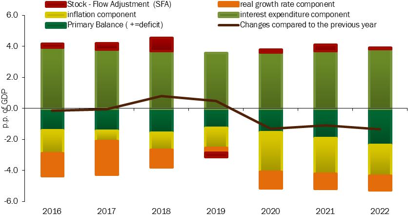
|
|
Source: From 2019, policy scenario
forecasts of the EFD.
|
In
2019, debt accumulation is fully explained by the snowball effect, which is positive and growing due to the
slowdown in nominal growth and an interest-expenditure component stable at 3.6 percent of GDP. In fact, in
2019, a sign reversal is expected in the stock-flow component, which results in a reduction of about 0.3
points of GDP, also due to the effect of the assumptions on proceeds from privatisation.
The
trend reversal in debt-to-GDP ratio is expected in 2020, with a value of 131.3 percent, due to a sharp decline
expected in public sector borrowing requirement of 2.4 percent of GDP (about 0.7 percentage points of GDP less
than in 2019) and a nominal growth accelerating to 2.8 percent.On the other hand, in
___
1 Discrepancies, if any, are
due to rounding.
2 Discrepancies, if any, are
due to rounding.
|
MINISTRY OF ECONOMY
AND FINANCE
|
63
|
|
ECONOMIC AND FINANCIAL DOCUMENT - SECT. I STABILITY PROGRAMME
|
2020 the primary
surplus will improve by around 0.3 percentage points of GDP, while the snowball effect is expected to
reduce significantly, thanks to the growth of nominal GDP and the stabilisation of interest. The decrease
in the level of debt also derives from the further reduction in the Treasury’s cash availability by around
0.1 percent of GDP and from the proceeds expected from privatisation and other financial gains for 0.3
percentage points of GDP, in line with the assumptions made in December 2018.
In 2021, the debt-to-GDP ratio will continue to decline, settling at 130.2 percent. The improvement
compared to 2020 (around 1.1 percentage points) is due, all other factors being equal, to the reduction in
public sector borrowing requirement of around 0.4 percentage points of GDP30 and to the expected 2.6 percent increase in
nominal growth. The snowball effect and the stock-flow component will contribute to an increase in the
debt-to-GDP ratio, while the primary surplus will act in the opposite direction and will continue to
improve, instead, to 1.9 percent of GDP.
A further reduction in the debt-to-GDP ratio is expected in 2022, down to 128.9 percent, confirming
the downward trend beginning in 2020. The drop will be substantially in line with the previous year,
despite the marked reduction in the borrowing requirement (by about 0.8 percentage points of GDP) and a
nominal growth slightly down to 2.3 percent. The reduction in debt-to-GDP ratio compared to the previous
year is explained by an increase in the primary surplus, reaching 2.3 percent of GDP, from a change in
composition of the overall effect of stock-flow adjustment and of the snowball component. In particular,
the decrease in stock-flow component will offset almost all the increase in the snowball component,
explained in turn by the renewed increase in interest expenditure accompanied by lower growth.
Net of Italy’s shares of the loans to the EMU Member States (bilateral or through the EFSF) and of
the capital contribution of the ESM, the 2018 final debt-to-GDP ratio stood at 128.8 percent of GDP and it
is estimated that it will fall to 125.9 percent of GDP in 2022.
___
30 For more detail
on public sector account forecasts, see Section II of the EFD.
|
64
|
MINISTRY
OF ECONOMY AND FINANCE
|
|
III. NET BORROWING AND PUBLIC DEBT
|
|
TABLE III.10: PUBLIC DEBT DETERMINANTS
(in percentage of GDP) (1)
|
|||||
|
2018
|
2019
|
2020
|
2021
|
2022
|
|
|
Level (including
support) (2)
|
132.2
|
132.6
|
131.3
|
130.2
|
128.9
|
|
Changes compared to
previous year
|
0.8
|
0.5
|
-1.3
|
-1.1
|
-1.3
|
|
Factors that
determine the variations in public debt:
|
|||||
|
Primary surplus
(accrual)
|
-1.6
|
-1.2
|
-1.5
|
-1.9
|
-2.3
|
|
Snowball effect
|
1.5
|
2.0
|
0.0
|
0.4
|
0.9
|
|
of which: Interest (accrual)
|
3.7
|
3.6
|
3.6
|
3.7
|
3.8
|
|
Stock-flow
adjustment
|
0.9
|
-0.3
|
0.2
|
0.4
|
0.1
|
|
of which: Difference between cash and accruals
|
0.2
|
0.4
|
0.0
|
0.0
|
-0.8
|
|
Net accumulation of financial assets (3)
|
0.2
|
-0.7
|
0.0
|
0.3
|
0.5
|
|
of which: Privatisation proceeds
|
0.0
|
-1.0
|
-0.3
|
0.0
|
0.0
|
|
Impact of debt valuation
|
0.2
|
-0.1
|
0.2
|
0.2
|
0.3
|
|
Other (4)
|
0.3
|
0.0
|
0.0
|
-0.1
|
0.0
|
|
p. m. Implicit
Interest rate on debt
|
2.9
|
2.8
|
2.8
|
2.9
|
3.0
|
|
1) Discrepancies, if any, are due to rounding.
2) Inclusive of shares relevant to Italy of loans to the EMU Member States, (bilateral
or through the EFSF) and of the capital contribution of the ESM. Throughout 2018, the amount of
these shares was equal to approximately 58.2 billion, of which 43.9 billion for bilateral loans
and loans through the EFSF and 14.3 billion for the ESM programme (see Bank of Italy,
'Statistical Bulletin - public finance, borrowing requirement and debt' of March 15, 2019). The
estimates consider proceeds from privatisation and other financial income totalling 1 percent of
GDP in 2019, 0.3 percent of GDP in 2020 and 0 in subsequent years. In addition, a reduction in
MEF liquidity stocks is assumed of 0.1 percent of GDP for each year from 2019 to 2021. The
interest rate scenario used for the estimates is based on the implicit forecasts resulting from
the forward rates on the Italian government bonds for
the period of compilation of this present document.
3) Includes the effects of contributions for GLF and the ESM programme.
4) The item 'Other', residual compared to the preceding items, includes: variations in
MEF liquidity; statistical discrepancies; Eurostat reclassifications; contributions in support
of the Euro Area envisaged by the EFSF programme.
|
|||||
|
TABLE III.11: GENERAL
GOVERNMENT DEBT BY SUBSECTOR (1)
(in millions and in
percentage of GDP)
|
|||||
|
2018
|
2019
|
2020
|
2021
|
2022
|
|
|
Level including Euro Area financial support (2)
|
|||||
|
General government
|
2,321,957
|
2,359,097
|
2,401,013
|
2,442,577
|
2,473,609
|
|
% GDP
|
132.2
|
132.6
|
131.3
|
130.2
|
128.9
|
|
Central government (3)
|
2,245,888
|
2,285,396
|
2,329,784
|
2,373,801
|
2,407,326
|
|
Local government (3)
|
126,096
|
123,728
|
121,257
|
118,804
|
116,312
|
|
Social security funds
|
126
|
126
|
126
|
126
|
126
|
|
Impact of support in % GDP (4)
|
3.3
|
3.3
|
3.2
|
3.1
|
3.0
|
|
Level excluding Euro Area financial support (2)
|
|||||
|
General government
|
2,263,726
|
2,300,866
|
2,342,915
|
2,384,872
|
2,416,404
|
|
% GDP
|
128.8
|
129.4
|
128.1
|
127.2
|
125.9
|
|
Central government (3)
|
2,187,656
|
2,227,164
|
2,271,686
|
2,316,096
|
2,350,121
|
|
Local government (3)
|
126,096
|
123,728
|
121,257
|
118,804
|
116,312
|
|
Social security funds
|
126
|
126
|
126
|
126
|
126
|
|
1) Discrepancies, if any, are due to rounding.
|
|||||
|
2) Inclusive or exclusive of shares relevant to Italy of loans to the EMU Member States,
(bilateral or through the EFSF) and of the capital contribution of the ESM. Throughout 2018 the
amount of these shares was equal to approximately 58.2 billion, of which 43.9 billion for
bilateral loans and loans through the EFSF and 14.3 billion for the ESM programme (see Bank of
Italy 2018 Statistical Bulletin - public finance, borrowing requirement and debt' of March 15,
2019). The estimates consider proceeds from privatisation and other financial income totalling 1
percent of GDP in 2019, 0.3 percent of GDP in 2020 and 0 in subsequent years. In addition, a
reduction in MEF liquidity stocks is assumed of 0.1 percent of GDP for each year from 2019 to
2021. The interest rate scenario used for the estimates is based on the implicit forecasts
resulting from the forward rates on the Italian government bonds for the period of compilation
of this present document.
|
|||||
|
3) Including liabilities towards the other sub-sectors.
4) Including the effects of the Italian contribution in
support of the Euro Area: contributions to Greek Loan Facility (GLF) programme, EFSF and ESM.
|
|||||
|
MINISTRY OF ECONOMY
AND FINANCE
|
65
|
|
ECONOMIC AND FINANCIAL DOCUMENT - SECT. I STABILITY PROGRAMME
|
|
FIGURE III.2: TREND OF THE DEBT-TO-GDP RATIO (inclusive and exclusive of
support to Euro Area Countries)
|
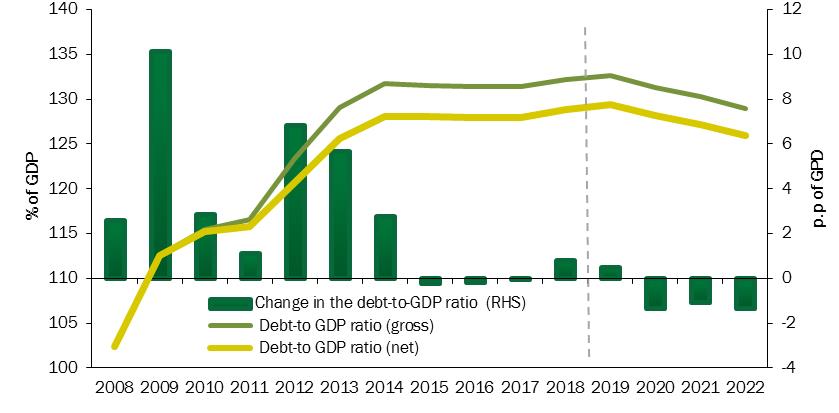 |
|
Source: ISTAT and
the Bank of Italy. From 2019, policy scenario forecasts.
|
III.5 THE DEBT RULE AND THE OTHER RELEVANT FACTORS
It is important to ensure the sustainability of public debt and aim towards its gradual
reduction, especially if it assumes particularly high values in relation to GDP. In such
circumstances, debt takes away important resources from public finance, because they are allocated to
paying interest, and is a burden for future generations. The objective of debt reduction can be
achieved on the one hand by investing in economic growth (and hence on the ratio denominator), and on
the other hand by improving the balance sheet in public accounts31 through a careful budgetary policy.
European regulations require the planning of public budgets to ensure over time the achievement
of a debt-to-GDP ratio of 60 percent following a rule that dictates the timeline for the reduction.
The European Commission, as part of its supervisory role, is called upon to assess compliance with
this rule as laid down in general by the Treaty on the Functioning of the European Union (TFEU) (see
box ‘The Debt Rule’).
In recent years, the deep economic crisis and the weakness of the recovery, in a context of low
inflation, discouraged manoeuvres of fiscal adjustment that were too pronounced and ultimately would
have been deflationary and counter-productive in terms of debt dynamics. Therefore, since the rule was
established, Italy has rarely presented a public finance plan that is formally in line with it.
___
31 The dynamics
of debt are also affected by the capital proceeds and other items that reduce the general government
borrowing requirement.
|
66
|
MINISTRY OF ECONOMY AND FINANCE
|
|
III. NET BORROWING AND PUBLIC DEBT
|
Since 2015, the European Commission has found that the dynamics of Italian public
debt were - prima facie - non-compliant with the debt
rule. Having initiated dialogue with Italy, the Commission has repeatedly and substantially accepted
the reasons put forward by the Italian Government for failing to comply with the debt rule and
decided not to launch infringement proceedings. According to the Commission’s interpretation,
compliance with the preventive arm of the Stability and Growth Pact and the adoption and
implementation of appropriate reforms to increase potential growth and improve debt sustainability
played to Italy's advantage. In one case (in 2017), however, the Commission did ask to make a
structural correction to the public accounts in order to ensure convergence towards the MTO. The
recommendation was implemented by the Italian Government, which presented, at the same time as the
adoption of the EFD 2017, a package of measures designed to reduce the structural deficit32.
|
F
O
C
U
S
|
The debt rule
The debt
rule was introduced to European Regulation from the so-called Six Pack and was transposed at
national level with the implementing law of the principle of budgetary equilibrium in the
Constitution (Law No. 243/2012). Fiscal discipline on debt became fully operational in 2015,
after a period of transition started for Italy in 2012, with the exit from the procedure for
excessive deficits.
The debt
rule requires that, in order to ensure the debt-to-GDP ratio is reduced at a satisfactory
pace towards the threshold of 60 percent of GDP, the programming of the public budget must
comply with at least one of the following criteria:
a. the part of debt in excess of the
reference value of 60 percent of GDP should be reduced on an annual basis to 1/20 of the
average of the values of the three years prior to the current value (backward-looking
criterion) or in the two years following the year of reference (forward-looking
criterion).
b. the excess debt in relation to the
backward-looking benchmark must be attributable to the economic cycle (using an index that
expresses the debt-to-GDP ratio that would have been obtained if in the preceding three
years the numerator had been adjusted according to the impact of the economic cycle and
the nominal GDP denominator had grown at the same pace as the potential GDP).
Starting
from the 2016 Stability Programme, compliance with the debt rule based on the
backward-looking configuration or that adjusted according to the economic cycle is fully
evaluated for the consolidated data provided by ISTAT (the Italian National Statistics
Bureau). The evaluation of the debt rule is carried out in relation to the more favourable
benchmark determined based on the criteria described above. Based on current data, the more
favourable benchmark proves to be the forward-looking benchmark in which compliance with the
rule in the reference year is measured by quantifying the gap produced on the basis of the
debt-to-GDP projections for the two subsequent years.
If from
initial analysis there is evidence of non-compliance with the debt or deficit rule, the
Commission prepares an in-depth report pursuant to art. 126.3 of the Treaty on the
Functioning of the European Union (TFEU), in which all the factors33 justifying
the deviation
|
___
32
Measures included in Decree Law No. 50/2017 converted into Law No. 96/2017, O.J. 144/2017.
33
European legislation establishes that the Commission can desist from launching proceedings for
excessive deficit, taking account of the existence of relevant factors such as: the medium-term
economic situation, compliance with the rules dictated by the stability and growth pact, the trend
and sustainability of public debt in
|
MINISTRY OF
ECONOMY AND FINANCE
|
67
|
|
ECONOMIC AND FINANCIAL DOCUMENT - SECT. I STABILITY PROGRAMME
|
|
are
considered. On this occasion, the country under observation can send its own reasons
justifying the failure to achieve the required fiscal consolidation. In issuing its opinion,
the Commission may conclude that, because of an overall assessment, the country is not found
to be in deviation and does not therefore recommend the launch of excessive deficit
proceedings.
From 2015, the first year in which the European
Commission drew up the report pursuant to art.126.3 of the Treaty in relation to Italy,
the choice of Italian Governments was to draw up and publish a very detailed analysis of
the factors explaining the evolution of public debt and the failure to reach the benchmark34. For a summary of the dialogue between 2015 and 2017, refer to
the box entitled ‘The debt rule and the report on the relevant factors’ found on page 52
of the 2018 EFD Update Memorandum. The assessment carried out by the European Commission
in May 2018 is treated in the following box ‘Judgement of the European Commission on
compliance with the debt rule’.
|
The ‘window of evaluation’ for the debt profile is still open for the three-year
period 2017-2019. In May 2018, the Commission found that the stock of Italian debt in 2017 was above
the reference threshold of 60 percent of GDP established by the Treaty. At the same time, in
addition to failing to achieve the reduction objectives imposed by the debt rule for 2017, the
projections for the years 2018 and 2019 seemed to confirm the failure of the adjustment for the
following years too. In its spring judgement, the Commission upheld that the cyclical conditions of
the Italian economy had improved and that therefore the weak economic recovery could no longer be
cause of the failure to adjust to the forward-looking benchmark. However, ex post compliance was acknowledged in 2017 of the preventive arm of the SGP in
relation to convergence towards the MTO and progress was recognised in the adoption and
implementation of the structural reforms in support of growth. Based on these considerations, Italy
was not in violation of the debt rule. However, the Commission recommended to achieve a more
pronounced fiscal adjustment for 2018, in order not to deviate from the path of convergence towards
the MTO35. A new evaluation was to be carried out at the time
of the presentation of the Draft Budgetary Plan in October 2018.
The Draft Budgetary Plan 2019, presented in October 2018, demonstrated the
Government's intention to follow a more expansive fiscal approach compared with the balances at
unchanged legislation, i.e. the public finance scenario inherited from the previous legislature. The
decision came from the desire to implement gradually the Government programme, funding significant
and particularly qualifying operations, and to resume spending for investments. This change in
budgetary policy led the Commission to question its judgement on compliance with the debt rule for
2017. In particular, the Commission noted a significant
the medium term. In addition, each Member
State may propose to the Council and the Commission specific factors justifying the deviation from
compliance with the rules.
34
The analyses drawn up by the government and the reports pursuant to article 126(3) of the Treaty can
be consulted in chronological order at the following link: https://ec.europa.eu/info/business-economy-Euro/economic-and-fiscal-policy-coordination/eu-economic-governance-monitoring-prevention-correction/stability-and-growth-pact/corrective-arm-excessive-deficit-procedure/closed-excessive-deficit-procedures/italy_en.
35
Recommendation of the Council of the European Union of 13 July 2018 on Italy's 2018 national reform
programme and formulating a Council opinion on the Italian stability programme for 2018: https://eur-lex.europa.eu/legal-content/IT/TXT/PDF/?uri=CELEX:32018H0910(11)&from=EN
|
68
|
MINISTRY OF ECONOMY AND FINANCE
|
|
III. NET BORROWING AND PUBLIC DEBT
|
deviation
from the structural effort of 0.6 percent of GDP required in 2019 in order to converge towards the
MTO.
The reservations expressed by the Commission gave rise to an intense phase of
dialogue between the two parties, as provided for by EU law (refer to focus ‘Dialogue with the
European Commission on the 2019 Draft Budgetary Plan’ in para. III.2). In addition to the request
for clarification on the DBP, the Commission considered it appropriate to update the report on the
relevant factors pursuant to art. 126.3 of the Treaty. As a result of this, Italy sent a new Draft
Budgetary Plan, reiterating the public finance objectives, and responded to the requirement to
justify the reasons for the failure to comply with the debt rule (see box ‘Judgement of the
European Commission on compliance with the debt rule’). The Commission report of November 201836 drawn up pursuant
to art. 126.3 of the Treaty nevertheless concluded that the relevant factors put forward by Italy
were not sufficient to justify deviation from the path indicated by the debt rule. Consequently,
the Commission believed there was due justification for opening an excessive deficit procedure.
The dialogue between the Commission and the Government in the weeks that
followed enabled the negotiation of a new public finance convergence path that reconciled the
demands of public finance sustainability with the Government Contract objectives37. This negotiation
prevented the opening of an infringement procedure and postponed the assessment in the spring of
2019 as foreseen by the calendar of the European semester.
|
F
O
C
U
S
|
The judgement of the European Commission on the debt
rule
In its
overall assessment on the evolution of Italian public debt conducted pursuant to art.
126.3 of the TFEU and published in May 2018, the Commission had concluded that the debt
criterion should be considered respected for the moment. The Commission pointed out the
need to implement higher fiscal adjustment for 2018 in order to ensure the path of
convergence towards the MTO. In November, the Commission decided to re-examine compliance
with the debt rule with an update of the report pursuant to art. 126.3 of the Treaty. The
expansive revision of the public finance objectives included in the 2019 Draft Budgetary
Plan had changed the information base on which the judgement of May 2018 was delivered. In
particular, the deterioration of the structural deficit for 2019 announced by the
Government was going in the opposite direction to the fiscal consolidation indicated by
European rules.
In response, the Government therefore put forward a series of
important factors in support of an overall assessment (including quality) of the trend
in public accounts and debt. The first factor is the cyclical situation: in 2018, the
Euro area suffered a slowdown in exports and industrial production; the Italian
manufacturing industry was hard hit by the decline in international trade and the
increasing wave of protectionism. This cyclical situation is added to years of weak
growth during which the restrictive fiscal policies have improved the numerator of the
debt-to-GDP ratio through increasing primary surpluses but have not contributed to
revitalising the denominator (i.e. nominal GDP). In fact, the economy has found it
difficult to return to its full potential, with high rates of unemployment and low
|
___
36 European
Commission report drawn up pursuant to art. 126.3 https://ec.europa.eu/info/sites/info/files/economy-finance/1263_commission_report_211118_-_italy_en_1.pdf
37
For a detailed report, see the focus ‘Dialogue with the European Commission on the 2019 Draft
Budgetary Plan’ in paragraph III.2.
|
MINISTRY OF
ECONOMY AND FINANCE
|
69
|
|
ECONOMIC AND FINANCIAL DOCUMENT -
SECT. I STABILITY PROGRAMME
|
|
inflation. The second important factor is focused on the fact that
the Italian economy suffers from a much wider output gap than that identified by the
methodology agreed at European level. Taking into account MEF estimates, the structural
budget is in line with the forecasts of the European fiscal regulations. The third
important factor is based on the urgent need to promote social inclusion and revitalise
public investment. The expansive approach of the fiscal policy proposal in the DBP 2019
supports own key measures such as Citizen's Income and ‘Quota 100’, as well as important
infrastructural investments. The measures, not only of a fiscal nature, envisaged by the
Government aim to stimulate both supply and aggregate demand. Another very important
factor is the fact that debt sustainability, using alternative measures of potential
growth, is not at risk in either the medium or long term. The nature of the public debt
characterised by long maturities and fixed rates ensures a certain resilience to the
volatility of the financial market. Moreover, Italy has a very low level of contingent
liabilities.
In fact,
in its final judgement, the Commission retained that the relevant factors presented by
the Italian Government were not sufficient to justify the failure to adjust public debt.
In particular: (i) the deterioration of macroeconomic conditions did not justify the gap
in relation to the reduction of the debt established by European rule, given the growth
of nominal GDP of more than 2 percent in 2016; (ii) the measures presented by the
Government were a step backwards compared to certain reforms implemented recently,
first and foremost in the area of pension expenditure; and, finally, iii) forecast data
of the Commission and data contained in the DBP2019 underscored the risk of a
significant deviation from the adjustment path towards the MTO recommended for 2018 and
the risk of serious non-attainment of the structural adjustment for 2019 of 0.6 percent
of GDP foreseen by the adjustment matrix agreed within the Stability and Growth Pact and
recommended by the Council to the Italian Government. Overall, therefore, the final
report suggested that the debt criterion as defined by the Treaty and by EC Regulation
No. 1467/97 was to be regarded as not respected and that this justified the launch of an
excessive deficit procedure.
|
The evolution of the debt-to-GDP ratio highlights a narrowing of the gap with
the path of convergence to the threshold of 60 percent in the forward-looking configuration for
2018 and 2019 of the cyclically adjusted debt for 2020. In detail, compliance with the rule for
2018 is assessed on the basis of the 2020 debt-to-GDP ratio forecast, which is 131.3 percent.
The debt rule indicates a convergence path that implies, in the forward-looking configuration, a
debt-to-GDP ratio of 125.1 percent. The gap with the forward-looking benchmark is therefore 6.2
percent of GDP (in any case more favourable than the other debt rule configurations). In the
same way, compliance with the rule in 2019 is evaluated using the forward-looking configuration.
In the policy scenario, the debt-to-GDP ratio would be at 130.2 percent that compared with a
benchmark of 125.1 percent to achieve in the forward-looking
configuration, points out a deviation of 5.2 percent. In 2020, the debt-to-GDP distance is
minimal in the cyclically-adjusted debt configuration, with a gap of 3.9 percent.
|
70
|
MINISTRY OF ECONOMY AND FINANCE
|
|
III. NET BORROWING AND PUBLIC DEBT
|
|
TABLE III.12 COMPLIANCE WITH THE DEBT RULE: FORWARD LOOKING CRITERION
AND CYCLICALLY ADJUSTED DEBT
|
||||||
|
Scenario
|
||||||
|
At unchanged legislation
|
Policy scenario
|
|||||
|
2018
|
2019
|
2020
|
2018
|
2019
|
2020
|
|
|
Debt in year t+2 (% percent of GDP)
|
131.7
|
130.6
|
129.6
|
131.3
|
130.2
|
128.9
|
|
Gap in relation to the forward-looking benchmark (% of GDP)
|
6.5
|
5.4
|
4.9
|
6.2
|
5.2
|
4.4
|
|
Gap in relation to cyclically adjusted debt (% of GDP)
|
8.2
|
7.3
|
4.0
|
7.9
|
7.1
|
3.9
|
Thus, the difficulty remains in complying with the debt rule, even in the
presence of a medium-term path to adjust both the nominal and structural deficit. In fact, the
economic policy pursued by the Government has to deal with lower nominal growth, caused by the
deterioration of the international macroeconomic scenario and a real cost of debt that is still
quite high. Consolidation manoeuvres that raise the primary surplus ex-ante prove once again to be counter-productive, assuming a pro-cyclical
nature. It should however be noted that growth projections are very cautious and reflect the
drastic revision of the prospects of international trade that could in future be revised
upwards. The impact of the reforms that will be implemented in the next few months by the
Government must also not be overlooked. It is then plausible to assume a fall in yields on
government bonds. A more favourable context would make it much easier to achieve compliance with
the debt rule.
|
F
O
C
U
S
|
Assessment of the impact of measures
relating to Citizen's Income and Quota 100 on
potential GDP and on the output gap
Pursuant
to the European and national legislation in force, the output gap contributes to the
quantification of the cyclically adjusted budget balance and thus to the estimate of the
so-called structural balance. This estimate is a crucial figure in assessing the
European Countries’ compliance with the fiscal rules enshrined in the Stability and
Growth Pact of the European Union and those in force nationally (for Italy, Law
243/2012). An overall assessment of the effects on the economy of the measures relating
to the Citizen's Income (RDC) and to the so-called Quota 100 (contained in Decree Law
No. 4/2019) was presented in a Focus of this Stability Programme and - in a more
articulated manner - in the National Reform Programme, to which we refer. This Focus
concentrates on the estimated impact of the two measures on potential GDP and on the
output gap.
The evaluation is carried out as follows: potential GDP and the
output gap (OG) corresponding to the scenario at unchanged legislation (which includes
the RDC and Quota 100) are calculated and to alternative ad hoc constructed scenarios.
These ad hoc scenarios refer to the macroeconomic scenarios obtained by subtracting
the effects on the economy of the cited measures, estimated using the ITEM econometric
model, from the scenario at unchanged legislation. Macroeconomic scenarios that
exclude the impact of the RDC, Quota 100 and both measures are considered separately.
The impact on potential GDP and on the output gap is thus calculated as the difference
between the estimates produced by the alternative scenario considered and those
produced by the scenario atunchanged legislation, i.e. estimated impact on OG = OG alternative scenario - OG at
|
|
MINISTRY OF
ECONOMY AND FINANCE
|
71
|
|
ECONOMIC AND FINANCIAL DOCUMENT
- SECT. I STABILITY PROGRAMME
|
|
unchanged legislation.
The
calculations made follow the official production function methodology38. One
evaluation component is found upstream of the financial year in the estimate of the
economic impact of the measures. The results obtained show that, overall, the measures
have a positive effect on potential growth; the impact is not immediate but spread
over time. The most important estimate for the purposes of European fiscal
surveillance, however, is not potential GDP, but the output gap; from this point of
view, it is estimated that the two measures have contributed to broadening it, but
only moderately.
Finally,
it is important to emphasize that the effects of the measures on potential growth are
not immediately detectable by performing a comparison between the estimates for the
macroeconomic scenario at unchanged legislation relating to this Stability Programme
and the estimates submitted in previous official documents. Potential GDP is a
function of the overall macroeconomic scenario and is influenced by the trend in gross
domestic product, in turn a function of a changing exogenous scenario of reference.
The
following Focus sections briefly illustrate the characteristics of the methodology for
estimating potential GDP and the output gap and then analyse the impact of the
measures, both separately and jointly. Particular attention is paid on the different
caveats underlying the estimates, a full understanding of which is crucial for
grasping the uncertainty of the precise estimates presented and the purely indicative
intention of the exercise.
Estimate of potential GDP and the output gap
The
output gap is defined as the distance between the real product (Y) of an economy and
its respective potential (
(1)
The
potential product is the maximum output obtainable from an economy without incurring
inflation and is therefore a non-observable (‘latent’) variable whose estimation
requires a theoretical model. The potential GDP estimation model perfected by the
European Commission is based on a Cobb-Douglas production function. The GDP of the
economy can be represented a product weighed using the factors of production: labour
(L), capital (K) and total factor productivity (TFP, so-called Solow residual). To
summarise
(2)
where
the weight of the labour factor (α) is set at 0.65.
According
to the methodology agreed at European level, the Labour factor is in turn obtained as
follows:
(3)
where
POPW is the population of working-age (15-74), PART is the participation rate, UR the
unemployment rate and HOURS the hours worked per employed individual.
To
switch from real GDP to potential GDP, the actual values (or forecast values for
future years) of the factors of production are replaced by the corresponding potential
values obtained through statistical filters that allow the trend component to be taken
out. In the case of the labour factor, all the variables of the (3) are filtered out
except POPW. The trend
|
___
38
It should be noted that the estimate is sensitive to the choice of some initial parameters,
such as the priors of TFP and the bounds of the NAWRU.
|
72
|
MINISTRY OF ECONOMY AND FINANCE
|
|
III. NET BORROWING AND PUBLIC
DEBT
|
|
in
PART and HOURS variables is obtained using a Hodrick-Prescott filter39. To
obtain the unemployment trend, on the other hand, a Kalman filter is used in which
the trend-cycle breakdown is ‘guided’ by an equation illustrating the relationship
between wage inflation and unemployment cycle (according to the Phillips curve
model). The value thus obtained corresponds to the NAWRU (Non-Accelerating Wage Rate
of Unemployment), namely the rate of unemployment to which economic theory
associates an absence of pressures of inflation. To summarise
(4)
Where
The
Capital factor is not filtered because it is assumed that the maximum contribution
to capital potential is given by the full use of the capital stock in an economy
(therefore
To
obtain the potential level of Total Factor Productivity, a Bayesian Kalman filter is
used in which the trend/cycle breakdown is guided by a composite variable of used
capacity (CUBS).
The
potential product is thus given by:
(5)
where
The effects of the measure using the official
methodology
Methodological premises
As
said above, the impact of the adoption of Decree Law No 4/2019 on the output gap is
relevant for considerations regarding the fiscal surveillance carried out within the
context of the European semester. It is the output gap, in fact, that is used for
the cyclical adjustment of the nominal budget balance and to obtain the structural
balance. It is therefore especially important to assess the impact on this value for
the reference year t (currently corresponding to 2019) and the following year
(2020): this is the two-year period subject to greater attention from the European
Commission. However, the effects on the year t-1 (2018)40 and on the last two years
of the planning horizon (2021-2022) are also significant for verifying the
convergence of the structural balance towards the Medium Term Objective.
Another
premise is that the effects of the measures only affect the different components of
the potential product gradually (labour and total factor productivity, as per
equation (5), given that there is a delay in the transfer of an increase in the
actual variables to their trend values (generated by statistical filters). By way of
example, Figure A shows that, considering an immediate and permanent rise in the
participation rate in 2019, its trend component
|
___
39
The Lambda value applied by the European Commission to filter PARTS and HOURS is 10.
40
It is recalled that a revision of potential growth estimates has an impact on the entire
estimate horizon, not just on the years subject to forecasting.
41
It should also be observed that a variation in PART also has an impact on the past values of
the variable  .
.
|
MINISTRY
OF ECONOMY AND FINANCE
|
73
|
|
ECONOMIC AND FINANCIAL
DOCUMENT - SECT. I STABILITY
PROGRAMME
|
|
trend variable is further delayed if the shock on PART is
modulated gradually over time rather than showing a sudden increase. It is also to
be noted that the different value of the participation rate implies a change of the
filtered variable even in the past (i.e. in the years prior to 2019).
|
|
FIGURE A: UNFILTERED SERIES OF PARTICIPATION (PART) RATE WITH
SHOCK OF 2.5 PP AND RELATIVE FILTERED SERIES
|
|
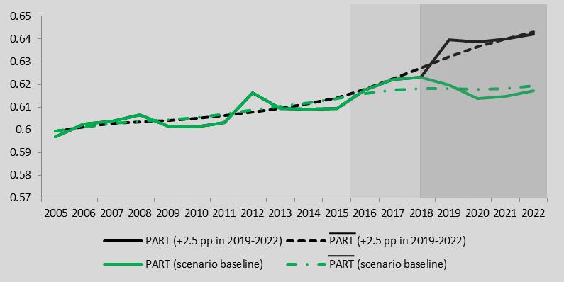 Source: MEF analysis.
|
|
Focusing
our attention on the output gap, as defined by (1) and observing the equations (2)
to (5), it may be inferred that the gap between
More
specifically, considering that the capital K is always equal to its potential value,
the output gap can be broken down into the sum of Labour gap and TFP gap (expressed
in logarithms). In turn, the Labour gap can be broken down into the sum of:
deviation between real hours worked and filtered total hours (HOURSGAP),
deviation between the real participation rate and filtered participation rate (PARTGAP) and
the deviation between unemployment rate and NAWRU (corresponding in (6) to UNEMPLGAP).
Therefore,
YGAP can be represented as follows:
(6)
Citizen's Income
We use this approach to assess, primarily, the effects of the
Citizen's Income. The rewarding element of the measure on the supply side consists
of introducing a proportion of inactive workers to the labour force by increasing
the rate of participation (PART) and, in part, the hours worked per employed
person (HOURS). At the same time, however, the measure also leads to an increase –
at least initially – in the unemployment rate. Those who receive the benefit must
declare themselves willing to work in the immediate future; at this point, no
longer inactive and not finding employment immediately, they would be classified
as
|
|
74
|
MINISTRY OF ECONOMY AND FINANCE
|
|
III. NET BORROWING AND PUBLIC
DEBT
|
|
unemployed42.
In
order to estimate the impact of the Citizen's Income on potential product and the
output gap, by using the official methodology, the potential output was estimated
in relation to a macroeconomic scenario that does not include the effects of the
measure. The estimates are compared with estimates relating to the scenario at
unchanged legislation that, instead, includes the effects of the measure. The
macroeconomic effects to be ‘subtracted’ from the scenario at unchanged
legislation are aligned with the evaluations performed using the ITEM econometric
model shown in the box in Chapter II, ‘An assessment of the macroeconomic impact
of Citizen's Income measures’.
Table
A shows the deviations between the two estimates of potential GDP and output gap
attributable to the measure. The first two rows show the deviations between the
actual and potential growth rates of the two scenarios, the remaining rows
indicate the deviations between the output gap and the different sub-components.
|
|
TABLE A: DIFFERENCE IN TERMS OF REAL GROWTH, POTENTIAL GROWTH, OUTPUT GAP
AND ITS COMPONENTS, BETWEEN SCENARIOS WITH AND WITHOUT CITIZEN'S INCOME
|
|||||||
|
2017
|
2018
|
2019
|
2020
|
2021
|
2022
|
||
|
Real
Growth
|
0.0
|
0.0
|
0.2
|
0.2
|
0.1
|
0.0
|
|
|
Potential
Growth
|
0.1
|
0.2
|
0.2
|
0.0
|
0.4
|
0.2
|
|
|
Output
gap
|
0.1
|
-0.1
|
-0.1
|
0.1
|
-0.2
|
-0.4
|
|
|
Labour
gap
|
0.0
|
-0.2
|
-0.4
|
-0.2
|
-0.3
|
-0.3
|
|
|
Unemployment gap
|
0.2
|
0.1
|
-0.1
|
-0.5
|
-0.5
|
-0.4
|
|
|
Hours worked gap
|
0.0
|
0.0
|
0.0
|
0.0
|
0.0
|
0.0
|
|
|
Participation rate gap
|
-0.2
|
-0.3
|
-0.2
|
0.3
|
0.2
|
0.2
|
|
|
TFP
gap
|
0.1
|
0.1
|
0.3
|
0.3
|
0.1
|
-0.1
|
|
|
The
scenario that includes the effects of the measure shows a higher GDP growth rate,
fully aligned with the ITEM evaluation, totalling on average around 0.15 percent
in the period 2019-2021. The variations in potential GDP are not immediately
aligned (year on year) to those in the underlying GDP and are, always on average,
greater. Reverse variations are also encountered for potential GDP, as can be
seen from the difference of 0.3 percentage points in potential growth in 2018 in
the scenario that includes the effects of the Citizen's Income.
The output gap increases in absolute value, becoming more
negative from 2017 and for the whole forecast horizon (with the exception of
2020). With reference to the financial year under examination, the broadening of
the output gap - denoted by minus signs Table A43 - is due to the
increase in the Labour gap. Within this Labour gap, the component that has the
greatest impact is the Unemployment gap. Figure B shows how, by comparing the
macroeconomic scenario that includes the Citizen's Income (‘with RDC’) and an
alternative scenario without the measure (‘without RDC’), a sudden increase in
the unemployment rate corresponds to a proportionally smaller variation in the
NAWRU. The increase in unemployment, greater than the increase in NAWRU, is
characterized as cyclical unemployment. In contrast, the Participation gap acts
in the opposite direction to the
|
___
42 The three conditions for classification as seeking
employment in the harmonized European data collection on the labour force are: 1) being
unemployed (a person is employed when he or she in the week of survey has done at least
one hour of paid work); 2) having actively sought work in the last 4 weeks; 3) being
available to start a job within two weeks from the week of the survey.
43 Negative numbers indicate a widening of the output gap
because the period considered starts with negative values, with GDP below its potential.
|
MINISTRY
OF ECONOMY AND FINANCE
|
75
|
|
ECONOMIC AND FINANCIAL
DOCUMENT - SECT. I STABILITY PROGRAMME
|
|
Unemployment
gap since the significant increase in participation rate is assigned by the HP
filter to the cyclical component (Figure C).
In
most of the simulation, the overall widening of the output gap compared to the
simulation without RDC is limited by a narrowing of the TFP gap. The upstream
evaluation performed using the ITEM model attributes to the measure a positive
variation in productivity as a result of its expansive effect; more precisely,
the increase in GDP is higher - in an initial phase - than the increase in
employment. However, once reflected in the production function methodology, the
increase in TFP is greater than that of its trend component.
|
|
FIGURE B:
COMPARISON BETWEEN THE UNEMPLOYMENT RATE SERIES IN SCENARIOS WITH AND WITHOUT
CITIZEN'S INCOME AND THE NAWRU SERIES IN SCENARIOS WITH AND WITHOUT CITIZEN'S
INCOME
|
|
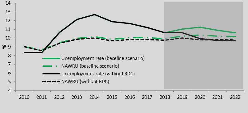 |
|
| Source: MEF analysis. | |
|
FIGURE C:
COMPARISON BETWEEN THE UNFILTERED AND FILTERED SERIES OF THE PARTICIPATION RATE
IN SCENARIOS WITH AND WITHOUT CITIZEN'S INCOME
|
|
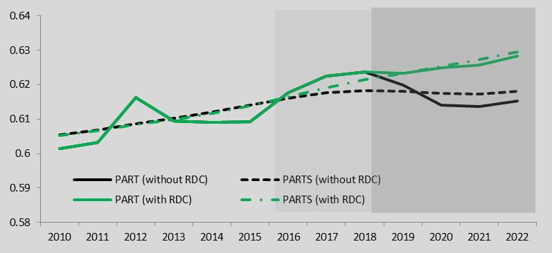 Source: MEF analysis.
|
|
Quota 100
Decree
Law No. 4/2019 in laying down urgent provisions on Citizen's Income and pensions
also provides for the introduction of a measure that allows access to retirement
for workers with at least 38 years of pension contributions and of at least 62
years of age (Quota 100), thus reducing the statutory retirement age.
|
|
76
|
MINISTRY OF ECONOMY AND FINANCE
|
|
III. NET BORROWING AND
PUBLIC DEBT
|
|
For the purposes of evaluating the potential, in order to
better interpret the results that will be shown, we will begin with certain
observations on the impact of the measure on the labour market. An initial and
immediate consequence is the reduction in participation in the age group
affected by the measure (elderly workers) and, in the absence of simultaneous
replacement recruitment; this would result in a corresponding reduction in
employment. However, the number of employed will tend to rise both due to the
effect of ‘replacement’ of retired workers (direct effect), and due to the
general impact of the measure on the economy (indirect effect).
This measure also was evaluated using ITEM (see the Focus
of Chapter II entitled ‘An assessment of the macroeconomic effects of pension
measures’). With reference to the variables that form part of the equation
(5), an initial indication is confirmation of the reduction in Labour factor L (lower employment and reduction of the
rate of participation). However, this effect decreases over time (between 2019
and 2022): in the first place, the lower participation is gradually offset by
a recovery in employment; secondly, the unemployment rate falls as early as
the first year44. Finally, the ITEM model estimates an effect of slight
expansion of the measure on economic growth: the fall in employment observed,
combined with an albeit slight increase in GDP, consequently generates an
increase in productivity (remember (2)).
The same approach used for the Citizen's Income is also
used to assess the impact of the Quota 100 on potential GDP and on the output
gap. In this case too, an alternative scenario to the scenario at unchanged
legislation is constructed using the ITEM evaluations. Table B shows the
effects estimated as the difference between the two potential variable
estimates. An initial result is that, overall, the reduced labour factor and
the increase in TFP offset one another and the effects on the potential
product are substantially neutral, with a slightly negative effect at the end
of the period.
|
|
TABLE B:
THE DIFFERENCE IN TERMS OF REAL GROWTH, POTENTIAL GROWTH , OUTPUT GAP AND ITS
COMPONENTS, BETWEEN SCENARIOS WITH AND WITHOUT QUOTA 100
|
|||||||
|
2017
|
2018
|
2019
|
2020
|
2021
|
2022
|
||
|
Real
growth
|
0.0
|
0.0
|
0.0
|
0.1
|
0.1
|
0.0
|
|
|
Potential
Growth
|
0.0
|
-0.1
|
-0.1
|
0.0
|
-0.1
|
-0.1
|
|
|
Output
gap
|
-0.2
|
-0.1
|
-0.1
|
0.0
|
0.2
|
0.3
|
|
|
Labour
gap
|
-0.1
|
0.1
|
0.0
|
-0.1
|
0.1
|
0.2
|
|
|
Unemployment gap
|
-0.2
|
-0.2
|
-0.1
|
0.1
|
0.3
|
0.3
|
|
|
Hours worked gap
|
0.0
|
0.0
|
0.0
|
0.0
|
0.0
|
0.0
|
|
|
Participation rate gap
|
0.1
|
0.2
|
0.1
|
-0.2
|
-0.2
|
-0.1
|
|
|
TFP
gap
|
-0.2
|
-0.2
|
-0.1
|
0.1
|
0.1
|
0.0
|
|
|
In this case too, what happens in terms of output gap is of
less immediate interpretation. The overall result is that, while in an initial
phase it expands, at the end of the period it decreases in absolute value. The
narrowing of the output gap - shown by positive values in the table - is due
in large measure to what happens to the Labour gap, and especially to the
|
___
44 The intuition behind this statement becomes clear by
observing the following identity relative to the unemployment rate (UR): UR=UNEMPL/ACTIVE=(ACTIVE-EMPLOYED)/ACTIVE (7)
With the numerator remaining unchanged (active
workers and those in employment will reduce by same amount), a reduction of the
denominator (active workers) leads to an increase in unemployment rate. However, even
a modest increase in workers in employment is enough to achieve a reduction in the
ratio. Given the current levels of unemployment and the number of active workers,
turnover needs to cover just 10 percent or more of the numbers going into retirement
to achieve a reduction in the rate of unemployment in the face of the retirement of an
actual 350,000.
|
MINISTRY
OF ECONOMY AND FINANCE
|
77
|
|
ECONOMIC
AND FINANCIAL DOCUMENT - SECT. I STABILITY PROGRAMME
|
|
Unemployment gap. The scenario that includes Quota 100
forecasts, as mentioned before, a progressive reduction in the unemployment
rate. However, only part of the reduction in unemployment rate is considered
structural (the reduction in the NAWRU is lower). This interpretation by the
production function methodology tends to narrow the Unemployment gap in
final simulated years. The increase in productivity recorded by the
simulations helps to raise the potential, by counteracting the effects of
labour component45. However, the TFP component helps to narrow
the output gap: the increase in productivity is considered largely cyclical
by the statistical filter used (the Kalman Filter).
|
|
FIGURE D: COMPARISON BETWEEN THE
SERIES OF THE UNEMPLOYMENT RATE AND THE NAWRU IN SCENARIOS WITH AND
WITHOUT QUOTA 100
|
|
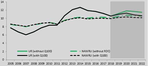 Source: MEF analysis.
|
|
Joint effects and conclusions
If the effects of both measures (Citizen's Income and
Quota 100) are considered together, by subtracting the overall effects of
the two measures estimated using ITEM from the scenario at unchanged
legislation, we obtain an intermediate result between the two presented. The
effects on the potential GDP and on the output gap tend to offset one
another but, as shown in Table C, there is a prevailing favourable effect on
the potential growth rate and we see an widening of the output gap in the
first years analysed and in 2022.
|
|
TABLE
C: THE DIFFERENCE IN TERMS OF REAL GROWTH, POTENTIAL GROWTH, OUTPUT GAP AND
ITS COMPONENTS, BETWEEN SCENARIOS WITH AND WITHOUT CITIZEN'S INCOME AND
QUOTA 100
|
|||||||
|
2017
|
2018
|
2019
|
2020
|
2021
|
2022
|
||
|
Real
Growth
|
0.0
|
0.0
|
0.2
|
0.2
|
0.2
|
0.0
|
|
|
Potential
Growth
|
0.1
|
0.1
|
0.1
|
0.0
|
0.3
|
0.2
|
|
|
Output
gap
|
-0.2
|
-0.4
|
-0.2
|
0.0
|
0.0
|
-0.2
|
|
|
Labour
gap
|
-0.1
|
-0.1
|
-0.3
|
-0.3
|
-0.2
|
0.0
|
|
|
Unemployment gap
|
0.0
|
0.0
|
-0.2
|
-0.4
|
-0.2
|
-0.1
|
|
|
Hours worked gap
|
0.0
|
0.0
|
0.0
|
0.0
|
0.0
|
0.0
|
|
|
Participation rate gap
|
0.0
|
-0.1
|
-0.1
|
0.1
|
0.1
|
0.1
|
|
|
TFP
gap
|
-0.2
|
-0.2
|
0.1
|
0.3
|
0.2
|
-0.2
|
|
___
45 In terms of effects on the potential, the greater
trend productivity offsets the effects of the reduction in jobs available. This
leads to the substantially neutral response just mentioned.
|
78
|
MINISTRY OF ECONOMY AND FINANCE
|
|
III. NET BORROWING AND
PUBLIC DEBT
|
|
The estimates presented are subject to various caveats.
Firstly, we note that the joint impact of the two measures is not linear,
i.e. the values in Table C are not exactly the sum of Tables A and B. This
is a characteristic of the methodology underlying the estimation of the
potential. It must also be pointed out that the results are ‘base
dependent’, i.e. the differences in potential observed between the base
scenario (in our case at unchanged legislation) and the comparison
scenario depend on the choice of base scenario. Therefore, starting from a
different macroeconomic scenario would change the results obtained, even
applying the same variations. The estimates are also a function of the
time interval over which the potential product is calculated;
traditionally, with a view to medium term planning, Italy goes as far as
year t+3; the Commission, on the other hand, stops at t+1 (or t+2 in the
case of Autumn Forecast). In conclusion, we recall the question of the
choice of the initial parameters to filter the original variables such as
the priors of TFP and the bounds of the NAWRU. The priors chosen are
consistent with those used to estimate potential GDP in this planning
document. We do not present here a systematic analysis of comparison with
the results obtained by choosing different priors; however, certain tests
performed gave similar results in terms of quality.
Medium-long term
impacts
For the purposes of assessing the impact of the
measures in question on potential GDP, we must consider the effects that
the measures, especially Citizen's Income, will have on the estimate of
the medium term parameter to which the structural unemployment tends to
converge (NAWRU ‘anchor’46 ), a parameter used to estimate
potential GDP in the short and medium term and in sustainability analysis.
Specifically, the amounts derived from the Citizen's
Income received by individuals recorded as unemployed who have declared
income from work within the preceding five years will be considered for
calculating the rate of replacement of unemployment benefits, used to
estimate the NAWRU anchor and positively correlated with this anchor. On
the other hand, structural unemployment is negatively affected by the
Active Labour Market Policies (ALMP), also used to estimate the anchor,
the scope of which is expected to grow due to the effect of the measure in
question. The combined effect of the two opposing trends can be estimated
by means of further analysis. Finally, we recall that analysis on the
effects of the measure, disregarding the context of estimating the NAWRU
anchor, are presented in the National Reform Programme.
|
___
46 In the medium term (t+10), the
value of the NAWRU is converged to an ‘anchor’ parameter obtained through a
regression panel that comprises 13 Member Countries of the European Union (‘old
Member States’). This parameter, re-estimated on each forecast round, affects both
the estimation of the short-term NAWRU (and therefore potential GDP and the output
gap) and medium-long term fiscal sustainability indexes. While the NAWRU
corresponds to the unemployment rate in the absence of inflationary pressures, the
anchor represents the long-term structural unemployment rate.
The regression panel obtains the anchor using
seven explanatory variables. The ‘structural’ variables are: Rate of Replacement
of Unemployment Benefit, Tax Wedge, Active Labour Market Policies Index, and Union
Density. The ‘non-structural’ variables are: Total Factor Productivity, Real
Interest Rate, and Construction Industry Cyclical Index.
|
MINISTRY
OF ECONOMY AND FINANCE
|
79
|
IV.
SENSITIVITY AND
SUSTAINABILITY OF PUBLIC FINANCES
IV.1 SHORT-TERM SCENARIOSThis section contains a short-term sensitivity
analysis of public finance targets in relation to different macroeconomic shocks.
Different approaches are used. The first part presents an analysis of the interest
expenditure sensitivity to shocks on the yield curve. Subsequently, the effects on
the debt-to-GDP ratio of shocks that simultaneously affect economic growth, the
primary balance and the yield curve are shown; the analysis in question is
performed via the stochastic simulation of the evolution of the debt-to-GDP ratio.
Finally, using a methodology developed by the European Commission, the overall
risk of fiscal stress for public finances is assessed; to do this, a risk index is
used that provides information on the probability of fiscal and macro-financial
crises in the short term (for the current year and the year immediately
following).
Sensitivity to interest rates
Year 2018 was particularly challenging for
public debt management, whose objective is to ensure financing of the borrowing
requirement of the State sector and the refinancing of maturing securities in
order to achieve an efficient risk-return combination. In fact, in marked
discontinuity with respect to 2017, year 2018 featured the predominant role of
both national and international geopolitical events, which mainly occurred in the
second half of the year. The contest between the USA and China on the issue of
duties, with a consequent slowdown in world trade, the political events that
marked the formation of the Italian Government after the national elections of 4
March 2018, as well as the preparation of the new government agenda, gave rise to
strong tensions on the government bond market with the consequent widening of the
yield differential with respect to the main countries of the euro zone and a
significant increase in the volatility of security prices. Although to varying
degrees, both phenomena persisted throughout the rest of the year with a
non-negligible impact on the issuance of new debt.
|
MINISTRY OF ECONOMY AND FINANCE
|
83
|
|
ECONOMIC
AND FINANCIAL DOCUMENT - SECT. I STABILITY PROGRAMME
|
The composition of the government bond stock
at the end of 2018 was largely in line with the trend of recent years, although
there were some more marked differences. Indeed, it is confirmed the reduction
in short-term instruments such as BOTs (approximately 0.1 percent), while
compared to the previous year, there was a slight increase in the share of
medium and long-term securities (approximately 0.3 percent), which is the result
of an increase in the medium-term component and a modest reduction in the
long-term component, as part of which, however, a new BTP benchmark with a
20-year maturity was issued.
The inflation-linked bond component, both
those linked to the HICP1, i.e. European inflation, and those linked to the
FOI2,
i.e. Italian inflation, recorded a slight increase (about 0.4 percent), as a
result of the increase in the share of both BTP Italia and BTP€i of the total
government bond stock. In fact, in 2018, two new BTP Italia bonds were issued
(May and November 2018) and a new BTP€i with a 5-year maturity (March 2018),
against zero maturities, although the linker segment was subject to repurchases
(approximately 4.5 billion euro), performed to ease the total number of
maturities in the coming years.
The variable-rate component indexed to the
6-month Euribor (CCTeu) decreased as compared to last year (by approximately 0.4
percent), as a result of market conditions that enabled lower issues in the
sector (down approximately 1.5 percent), to which were associated maturities
(for approximately 22 billion euro) and repurchases (for approximately 5.5
billion euro).
As in previous years, foreign securities
decreased (by approximately 0.2 percent), as a result of the lack of new issues
of international format during the year, due to market conditions that were not
favourable for this type of security, and the size of the maturities (for
approximately 3.5 billion euro).
Because of the market turbulence that occurred
in 2018, the issues made, although lower in absolute terms than in the previous
year, were characterised by certain discontinuities as compared to 2017, also
due to the lower volume of maturing securities. Short-term issues (BOTs)
increased (by approximately 2.3 percent), but it was above all in the area of
medium/long-term fixed-rate bonds that there were changes to the composition of
issues were found. In fact, although there was an increase (approximately 0.69
percent) in the number of instruments with maturities of 2-3-5 years, in
contrast to 2017, there was an increase in issuance in the 7-10 year segment (up
by approximately 1.37 percent) and a decrease in the segment with maturities
over 10 years (of approximately 2.6 percent).
___
1 Harmonised Consumer Price Index
for the euro area, excluding tobacco.
2 National index of consumer prices
for Families of Manual Workers and Non-Manual Workers, excluding tobacco.
|
84
|
MINISTRY OF ECONOMY AND FINANCE
|
|
IV. SENSITIVITY AND
SUSTAINABILITY OF PUBLIC FINANCES
|
The overall
average life of the government bond stock as at 31 December 2018 was 6.78
years, in line, although decreasing, with 2017, at 6.90 years and in any
case such as to continue to guarantee a low risk of debt refinancing and
exposure to sudden increases in issue rates. The Average Refixing Period
(ARP)3, the main index used to
measure interest rate risk, only slightly decreased from 5.76 years at the
end of 2017 to 5.67 years at the end of 2018 (the figure including
derivatives went from 6.25 to 6.11 years); the average financial duration of
the government bond stock went from 5.5 years at the end of 2017 to 5.3
years at the end of 2018 (the figure including derivatives went from 6.01 to
5.79 years). The decrease in the ARP is a consequence of the reduction in
the Average Life of Debt, which in part also justifies the decrease in
duration. In fact, as indicated above, although between 2018 and 2017 there
was a reduction in CCTeus on the public debt stock, the increase in market
interest rates on Italian government bonds, linked to the lower issues on
the sector with maturities of 15-50 years, more than offset the effect of a
reduction in the variable component, so much so as to determine a reduction
in the duration referred to above.
In line with previous years, in 2018 these
indexes thus indicate that the issuance policy has confirmed, in substance,
the results achieved in recent years in terms of reducing exposure to
refinancing and interest rate risks. As proof of this trend, sensitivity to
interest rates was analysed, an index that analyses the effects on interest
expense over the next four years (calculated on the SEC 2010 accruals basis),
deriving from a significant shock on the yield curve of government bonds. The
financial year was calculated considering the entire stock of government bonds
issued and the existing derivatives portfolio. Taking into account both the
current and future composition of the security stock, deriving from the
assumptions on issues and management consistent with those underlying the
estimates for interest expense, and assuming passive management of the
existing derivatives portfolio for the coming years, a permanent shock of 100
basis points was applied to the entire yield curve, as well as to the Euribor
rate, for the next four years.
The result shows an increase in interest
expenditure in relation to GDP of 0.12 percent in the first year, 0.27 percent
in the second year, 0.39 percent in the third year and 0.51 percent in the
fourth year. These results are broadly in line with those of the EFD 2018,
although with some slight increases4. These values therefore confirm
that the impact of a significant and permanent market shock on net debt
continues to be largely watered down over time.
The average cost at issuance in
2018 of 1.07 increased significantly compared to 2017 (0.68 percent) because
of the significant increase in the yield curve for
___
3 The Average Refixing Period
(ARP) measures the average time over which the debt becomes subject to market
interest rates. For zero coupon or fixed coupon bonds, this corresponds to the
residual maturity. For securities with variable coupons, this is the time
remaining until the next coupon is fixed.
4 It should be noted that
comparison with the EFD 2018 figures must take into account the fact that, in
this document, the financial year was calculated for the stock of domestic
securities, without taking into account foreign securities and the derivatives
portfolio. On the other hand, it should be noted that domestic securities as
at 31-12-2018 accounted for more than 97 percent of the stock of securities
issued and that, as at the same date, the notional value of the derivatives
portfolio was 5.6 percent of the same stock.
|
MINISTRY OF ECONOMY AND FINANCE
|
85
|
|
ECONOMIC AND FINANCIAL DOCUMENT - SECT. I STABILITY
PROGRAMME
|
Italian government bonds from mid-May onwards. However, this
new level is still very modest in relation to past figures.
The interest expenditure of the general
government sector, calculated according to the SEC 2010 accruals basis, stood
at just under 65 billion euro in 2018, a decrease of around 619 million euro
compared to the total figure for 2017. In terms of percentage of GDP, the
interest expense of general government in 2018 was 3.7 percent, a fall of 0.1
percent compared to the previous year.
|
FIGURE IV.1: INTEREST EXPENDITURE AS A PERCENTAGE OF GDP AND
WEIGHTED AVERAGE COST AT ISSUANCE
|
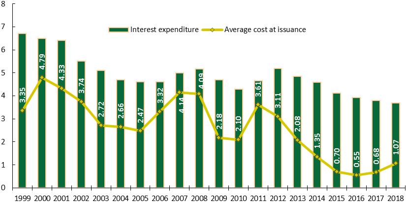
|
|
Source: MEF analysis.
|
The various components of the central
government aggregate reveal that domestic securities decreased by
approximately 121 million euro, foreign securities by 66 million and interest
bearing postal warrants (BPFs) pertaining to the MEF by approximately 582
million. Similarly to 2017, interest expenditure on instruments other than
securities instead increased, although to a lesser extent: interest on
liquidity stock held in the Treasury account by entities not part of the
general government increased by around 669 million euro, partly offset by the
reduction in other interest on government loans, which, unlike the previous
year, fell by around 336 million euro.
|
86
|
MINISTRY OF ECONOMY AND FINANCE
|
|
IV. SENSITIVITY AND SUSTAINABILITY OF PUBLIC FINANCES
|
|
FIGURE IV.2: TREND OF GOVERNMENT SECURITIES
YIELDS AT 1, 5 AND 10-YEAR MATURITIES
|
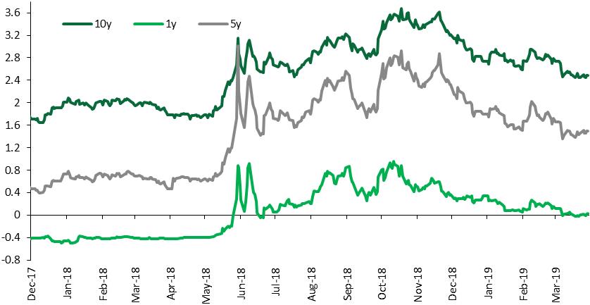 |
|
Source: MEF analysis.
|
|
FIGURE IV.3: BTP-BUND YIELD DIFFERENTIAL:- 10
YEAR BENCHMARK
|
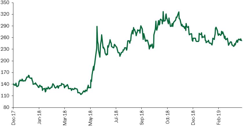 |
|
Source: MEF analysis.
|
The reduction in interest expenditure
deriving from government bonds (domestic and foreign) was very small, if
compared with the reduction in 2017 compared to 2016, which was around 1.4
billion euro. As described above, the changed conditions in the government
bond market led to a significant increase in the cost of debt at issuance in
2018: BOTs and CTZs were issued at positive rates, while higher European and
national inflation had a significant effect on indexed securities (BTP€i and
BTP Italia); for the entire nominal BTP segment, issues were made at cost
conditions in line with the increases in rates on the secondary market; only
CCTeus recorded a reduction in interest expenditure, of approximately 259
million euro, due to lower issues and maturities occurring
|
MINISTRY OF ECONOMY AND FINANCE
|
87
|
|
ECONOMIC AND FINANCIAL DOCUMENT - SECT. I STABILITY
PROGRAMME
|
during 2018. It follows from these considerations that,
despite the significant increase in the cost of new issues from the second
half of May, interest on the government bond stock suffered the
consequences only in terms of a smaller reduction compared to the previous
year: this result is almost entirely attributable to the structure of
outstanding securities, whose average life allows the effects of a sudden
increase in interest rates demanded by the market to be spread over a long
period.
The projected interest
expenditure estimates based on the policy scenario for the period
2019-2022, in line with the usual methodology, were prepared on the basis
of an interest rate scenario consistent with the expected rates implicit
in the Italian yield curve (forward rates) observed during the estimation
preparation period. Over the estimate period, the scenario assumes gradual
rate growth on all maturities, with a downward slope in the yield curve
that tends to decrease in the final years of the forecast.
The assumptions on European
and Italian inflation, necessary to estimate the impact on interest
expenditure of real securities (BTP€i and BTP Italia), were assumed to be
consistent with the macroeconomic policy scenario.
The forecasts for issues were
drawn up in such a way as to guarantee both the refinancing of maturing
securities and the payment of the borrowing requirements of the State
Sector, which are assumed to decrease over the estimate period: from 3.3
percent of GDP in 2019 to 1.4 percent of GDP in 2022.
Interest expenditure of the
general government, according to the SEC 2010 criterion, is estimated to
decrease slightly in 2019, by approximately 996 million euro, compared to
2018, mainly as a result of savings from government bonds indexed to the
HICP, by virtue of the expected inflation assumptions. In 2020, interest
expenditure appears to be in line with the previous year, at 3.6 percent
of GDP, or just 0.1 percent of GDP more than in 2019 due to the trend in
interest rates. This growth trend, although modest, has also been
confirmed in the last two years, amounting to 0.2 percent of GDP in both
2021 and 2022, which can be explained by the effect of the increase in
interest rates, by a significant volume of maturing bonds in both years
and by the cumulative effect of the borrowing requirements of the State
sector in the estimate period, which contribute to an increase in the debt
stock at the end of the forecast period.
The comparison with the
estimates prepared for the EFD in 2018, i.e. before the significant change
in market conditions that occurred in mid-May of the same year, shows that
this aggregate under unchanged legislation rose by 0.1 percentage points
of GDP in 2019 and 2020 and by 0.2 percentage points in 2022.
Stochastic simulations of debt
dynamics
In order to provide a
short-term sensitivity analysis of the trend in the debt-to-GDP ratio,
stochastic simulations were performed incorporating the historical
volatility of short and long-term interest rates and of economic growth in
nominal terms. The simulations were conducted using the Monte Carlo
method, applying shocks on interest rates and nominal growth to the
dynamics of the debt-to-GDP
|
88
|
MINISTRY OF ECONOMY AND FINANCE
|
|
IV. SENSITIVITY AND SUSTAINABILITY OF PUBLIC FINANCES
|
ratio for the policy scenario. These shocks are based on
the historical volatility of (short and long-term) yields and the nominal
GDP5 growth rate, and are obtained by performing 2000
extractions starting with a normal distribution with a zero average and
variance-covariance matrix observed over the period 1999-2018. This
approach therefore allows the uncertainty inherent in both yield curve and
economic growth forecasts to be taken into account simultaneously. More
specifically, there are two assumed cases: in the first, the interest rate
shocks are temporary; in the second, they are permanent. As regards the
shocks on nominal growth (always temporary), it is assumed that they also
have an impact on the cyclical component of the primary surplus. As a
result, for each projection year of the macroeconomic scenario and for
each type of interest rate shock (temporary and permanent) the
distribution of the debt-to-GDP ratio can be identified, represented as
probabilities using a fan chart (Figures IV.1A and 1B).
In the case of temporary
shocks, the debt is distributed around a median value equal to around 129
percent of GDP at the end of the time horizon. The uncertainty recorded
for the 2022 results is relatively low, as shown by a difference of about
15.4 percentage points between the tenth and ninetieth percentile of the
resulting distribution of the expected debt. The debt-to-GDP ratio shows a
downward trend from 2019 for the first 40 percentiles and from 2020 from
the fiftieth to the eightieth percentile. For the more severe shocks
(which are above the ninetieth percentile), the debt-to-GDP ratio is on
the increase, albeit slightly.
The permanent shock results
in a wider distribution of debt-to-GDP ratio values around the central
scenario, but assumes a similar dynamic to that obtained with temporary
shocks for the first sixty percentiles. Starting from the ninetieth
percentile, the dynamics of the debt-to-GDP ratio are on the increase. In
the case of permanent shocks, the uncertainty recorded for the 2022
results is higher, with a difference of around 17.6 percentage points
between the tenth and ninetieth percentile of distribution.
Compared to that reported in
the EFD 2018, the key difference in the simulations is due to the changed
forecast in dynamics of the debt-to-GDP ratio in the baseline scenario,
while the distribution of shocks around this scenario remains of similar
magnitude.
___
5 For further
information on the methodology adopted, see Berti K., (2013), ‘Stochastic
public debt projections using the historical variance-covariance matrix
approach for EU countries’, Economic Papers 480.
|
MINISTRY OF ECONOMY AND FINANCE
|
89
|
|
ECONOMIC AND FINANCIAL DOCUMENT - SECT. I STABILITY
PROGRAMME
|
|
FIGURE IV.4A: STOCHASTIC
PROJECTION OF THE DEBT-TO-GDP RATIO WITH TEMPORARY SHOCKS
|
FIGURE IV.4B: STOCHASTIC
PROJECTION OF THE DEBT-TO-GDP RATIO WITH PERMANENT SHOCKS
|
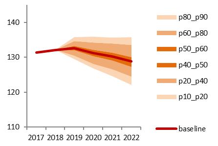 |
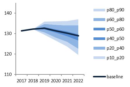 |
|
Note: The graphs show the 10th, 20th, 40th,
50th, 60th, 80th and 90th percentiles of the distribution of the
debt-to-GDP ratio obtained by stochastic simulation.
Source: MEF analysis.
|
|
In order to assess the
effects of the higher volatility of short and long-term interest rates
observed in the post-crisis period on the dynamics of the debt-to-GDP
ratio, the stochastic analysis was replicated, narrowing the period used
to extract the matrix of variance and covariance of the observed
interest rates and nominal growth. The new period covered is from 2008
to 2018. It has been found that, although the variability of the two
series of interest rates has increased, this effect is counteracted by
the decrease in variability of nominal growth. As a result, the
dispersion of the debt-GDP ratio around the median value remains broadly
identical to that of the simulations presented.
Overall
analysis of short-term fiscal risks
The European Commission has
introduced the S0 index to its sustainability analysis in order to
identify risks related to fiscal sustainability in the short term. The
analysis focuses on immediate risks, with a time horizon of about 12
months. The methodology differs from that used to quantify risks in the
medium and long term, described in the following sections, because no
fiscal gaps are taken into account. Rather, reference is made to a
composite probability index, built based on a wide range of fiscal and
financial variables that in the past have proven to offer early warnings
for episodes of stress.
|
90
|
MINISTRY OF ECONOMY AND
FINANCE
|
|
IV. SENSITIVITY AND
SUSTAINABILITY OF PUBLIC FINANCES
|
More precisely, the
methodology for constructing the S06 index is
based on a statistical signal extraction technique applied to 25
variables. A threshold is estimated for each variable that, when
reached, maximises the probability that the event will occur. The S0
index is calculated as a weighted average of the variables considered
(where the weights are given by their relative predictive capacity);
there are two sub-indices, one fiscal and one financial. The overall
value of the S0 index together with that of the sub-indices, compared
with their respective thresholds, are used to measure the probability
of an imminent shock. In particular, for the S0 index, a value above
the threshold indicates a potential risk in the short term, while
sub-index values above the thresholds indicate a risk concentrated in
the respective areas (fiscal or macro-financial).
With reference to the
values assumed by the index over time, it can be reported that, after
the peak reached in 2009 (0.58 the value of the overall S0 index), the
subsequent decrease, and further increase in 2012, the index time
series showed a marked decrease until 2015 (0.19 the value of the
overall S0 index). The index values until 2015 are not shown because,
starting from 2016, there was a discontinuity in the methodology; the
set of variables considered fell from 28 to 25 and the reference
threshold values were modified, making the results not fully
comparable.
Figure IV.5 shows how,
for 2017, the short-term risks were limited and down on the previous
year; these results had already been commented on in the previous
Economic and Financial Document. The overall index stood at 0.34
(compared to 0.42 in 2016), and remained below the threshold of 0.46,
above which the probability of a crisis occurring in the year
following the year of analysis would be considered high. The tax
component was 0.40, above the threshold of 0.36 (but with an
improvement as compared to 0.44 in 2016), while the macro-financial
component did not report problems and stood at a value of 0.31 (below
the threshold of 0.49 and a clear improvement compared to 0.40 in
2016), effectively counterbalancing the risk on the tax side, as
highlighted by the heat map (Table IV.1). The values of the 25
variables were fully updated for 2018, but the value of the S0 index
does not change because the position of each sub-component with
respect to the critical thresholds did not change. The results are in
line with that reported in the European Commission’s 20187 Fiscal Sustainability Report.
___
6 Berti, K., Salto, M. and Lequien, M., (2012), ‘An
early-detection index of fiscal stress for EU countries’, European
Economy Economic Papers No. 475.
7 See: European Commission ‘Fiscal
Sustainability Report 2018, Volume 2 – Country Analysis’,
Institutional Paper 094, https://ec.europa.eu/info/sites/info/files/economy-finance/ip094_en_vol_2.pdf.
|
MINISTRY OF ECONOMY AND FINANCE
|
91
|
|
ECONOMIC AND FINANCIAL DOCUMENT - SECT. I STABILITY PROGRAMME
|
|
FIGURE IV.5: THE S0
INDICATOR AND SUB-COMPONENTS
|
|
|
Source: MEF
analysis on 2019 EFD, AMECO, WEO, EUROSTAT data.
|
|
TABLE IV.1: HEAT MAP FOR
THE VARIABLES UNDERLYING THE S0 INDICATOR FOR 2018
|
|
Short-term risk from tax
variables
|
Net debt (%GDP)
|
Primary balance (%GDP)
|
Cyclically adjusted budget
balance (%GDP)
|
Stabilising primary balance
(%GDP)
|
Gross public debt
(%GDP)
|
Variation in public gross
debt (%GDP)
|
|
|
Net public debt
(%GDP)
|
Gross requirements
(%GDP)
|
Interest-growth
differential
|
Variation in public
expenditure (%GDP)
|
Variation in final
consumption of PA (%GDP)
|
Short term public debt
(%GDP)
|
||
|
0
|
1
|
0
|
0
|
1
|
1
|
||
|
Short-term risk from
macro-financial variables
|
L1. International net
investments (%GDP)
|
L1. Net savings of
households (%GDP)
|
L1. Private sector debt
(%GDP)
|
L1. Private sector credit
flow (%GDP)
|
L1. Short-term debt
of non-financial corporations (%GDP)
|
L1. Short-term debt
of households (%GDP) (*)
|
|
|
L1. Added value in the
construction sector (total %AV)
|
L1. Current account balance
(3-year backward moving average) (%GDP)
|
L1. Variation (3 years) in
REER (based on the export deflator)
|
L1. Variation in nominal
unit labour cost
|
Yield curve
|
Real GDP growth rate
|
GDP per capita in
PPP (%US$)
|
|
Note: The colours red and green indicate, respectively,
the variables above and below the optimal threshold,
calculated periodically by the European Commission and
published in the Debt Sustainability Monitor. The code L1
indicates that the variable is reported with the lagged value
of one period.
Source: MEF analysis.
|
|
92
|
MINISTRY OF ECONOMY AND
FINANCE
|
|
IV. SENSITIVITY AND
SUSTAINABILITY OF PUBLIC FINANCES
|
IV.2 MEDIUM-TERM
SCENARIOS
This section presents
the sensitivity analysis of the debt-to-GDP ratio based on
deterministic projection scenarios. A set of assumptions
(alternative scenarios) is used that collectively impact on GDP
growth, the yield curve and primary budget balances and allow the
extrapolation of the dynamics of the debt-to-GDP ratio over a
horizon extending to 2030.
Until 2022, the
reference scenario (or baseline) coincides with the policy scenario
of this Economic and Financial Document. In the medium term,
economic growth is aligned with that of potential GDP and the
primary balance in relation to GDP is maintained at the value
forecast for 2022; the annual interest expenditure which, in
addition to the primary surplus of the general government, is used
to estimate the dynamics of the debt, is calculated using the SAPE
model of the Treasury, which is fed by the database of the stock of
current and forecast government bonds. The debt-to-GDP ratio is
extended by taking as a starting point the composition and maturity
structure of the underlying debt stock in the last year (2022) of
the EFD.
The sensitivity
analysis is aimed at outlining the possible alternative path of debt
dynamics over the next ten years, assuming different growth profiles
in relation to different interest rate assumptions.
Therefore, an
optimistic and a pessimistic scenario are constructed around the
baseline scenario, based primarily on alternative assumptions for
the trend of the yield curve for public debt securities. In the
short term (time horizon of the EFD macroeconomic scenario), the
impact of the sensitivity assumptions is estimated by the Treasury's
macroeconomic model (ITEM). Unlike the sensitivity exercises
presented in the latest planning documents, the variations in rates
have an endogenous impact on nominal growth and therefore on the
primary surplus of the general government8. In the
medium term, the assumptions underlying the analysis are more
stylised so that gross domestic product growth is affected by
exogenous alternative assumptions on the behaviour of total factor
productivity (TFP) and the structural unemployment rate (NAWRU).
As regards the
characteristics of the different scenarios in terms of assumptions
on the yield curve, it is noted first that the baseline scenario
incorporates the current levels of market rates and the consequent
forward rates implicit in the current yield curve. Moreover, in the
elaboration of estimates, precisely from a prudential point of view,
the slope of the yield curve - calculated starting from the forward
rates - on very long maturities ranging from 30 to 50 years was
modified, bringing it back to the average levels found on the market
since the introduction of the 50-year maturity. In other words, the
current reversal between 30 and 50 years arising by considering only
forward rates has been eliminated from the generation of future
rates; this reversal has indeed never been matched in the actual
market data of forward rates beyond two years of existence of the
50-year maturity.
___
8 Within the Treasury Department's econometric
model, a rise in long-term rates, assuming that German rates remain
at baseline level, leads to an increase in the spread. Financial
restriction is triggered through the channel of rates charged by
banks to their customers and this has a depressive effect on demand.
Lowering rates, of course, has the opposite effect.
|
MINISTRY OF ECONOMY AND FINANCE
|
93
|
|
ECONOMIC AND FINANCIAL
DOCUMENT - SECT. I STABILITY
PROGRAMME
|
In the optimistic
scenario, a parallel reduction of the entire Italian government
bond rate curve of 100 basis points is assumed at the end of 2019,
to remain unchanged in the subsequent period. Conversely, in the
pessimistic scenario, the yield curve is assumed to rise by 100
basis points in parallel at the end of 2019 and for the entire
forecast period. For both high and low growth assumptions, in
December 2022 rates start to converge again at baseline level and
remain anchored to the baseline from then on.
|
F
O
C U S |
Medium-term sensitivity assumptions
The medium-term simulations
presented below include:
i) A baseline scenario that
incorporates, in the period 2019-2022, the real and
potential GDP growth rates of the macroeconomic scenario
underlying this Economic and Financial Document. For the
years following 2022, in line with the ‘T+10’ methodology
currently used by the European Commission and discussed at
the EPC-Output Gap Working Group (OGWG), the growth rate
of the potential product is projected according to the
production function model, extrapolating the variables
related to the individual production factors using
statistical techniques (e.g. the Total Factor
Productivity, TFP, which in 2030 reaches a growth rate of
around 0.5 percent) or assuming that they converge in 2030
towards structural parameters (e.g. the Non-Accelerating
Wage Rate of Unemployment, NAWRU, which converges to an
anchor value of around 9.76 percent, as shown in Table
R.1). The output gap closes following a linear trend in
the three years following 2022 (it closes to zero in
2025). Again since 2022, the yield curve remains constant
until the end of the forecast horizon, while the growth
rate of the GDP deflator and the inflation rate calculated
on the consumer price index converge to 2.0 percent in
20259. Moreover, in line with the
assumption of unchanged policies, the cyclically-adjusted
primary balance for 2022 remains constant at the reference
level of 2.4 percent of GDP until 2030.
ii) A pessimistic scenario that
assumes a sudden increase in the yield curve of around 100
basis points above the reference scenario curve. This
shock is reabsorbed at the end of 2022. From 2022, the
yield curve remains constant until the end of the forecast
horizon. As a result of the increase in the interest rate
curve as compared to the reference scenario, GDP growth
decelerates by 0.03 in 2019, 0.3 percentage points in 2020
and 0.4 in 2021 and 202210.
The potential GDP series for the years 2019-2022 is
obtained by applying the usual methodology of the
production function agreed at European level11. From 2022, the NAWRU sets
off on a convergence path that ends in 2030 at 1
percentage point above the baseline scenario anchor, while
the TFP growth rate converges to 0.5 percentage points
below the baseline scenario level in 2030, i.e. at a
negative value of 0. The output gap closes following a
linear trend in 2025. Because of lower growth, the primary
surplus12 decreases
correspondingly in the period 2019-2022 and subsequently
remains constant at its structural level until the end of
the forecast horizon. The growth rate of the GDP deflator
and the rate of consumer price inflation converge to 2.0
percent in 2025.
iii) An optimistic scenario that
assumes a sudden reduction in the yield curve of 100 basis
|
___
9 In the three simulation scenarios, the
inflation rate is invariably expected to converge to the policy
objective of 2 percent, because the growth path is always assumed
to align itself with the potential path by 2025.
10 With regard to the impact of sensitivity
assumptions in the short term, the Treasury macroeconometric model
(ITEM) estimates that the exogenous variation in interest rates
affects economic growth through the channel of domestic demand,
i.e. investments and consumption.
11 See in this regard the Methodological Note
annexed to Section III1 of the EFD 2019.
12 For more details on how the alternative
series of the primary surplus in the high and low growth scenarios
is obtained, see the Methodological Note annexed to Section III.3
of the EFD 2019.
|
94
|
MINISTRY OF
ECONOMY AND FINANCE
|
|
IV.
SENSITIVITY AND SUSTAINABILITY OF PUBLIC FINANCES
|
|
points below the reference
scenario curve. This shock is reabsorbed at the end of
2022. From 2022, the yield curve remains constant until
the end of the forecast horizon. Because of the decrease
of the curve of interest rates, compared to the
reference scenario, GDP grows by additional 0.03
percentage points in 2019, 0.3 percentage points in 2020
and 0.4 in 2021 and 2022. The potential GDP series for
the years 2019-2022 is obtained by applying the
production function methodology agreed at European
level. From 2022, the NAWRU sets off on a convergence
path that ends in 2030 at a value of 1 percentage point
lower than the baseline scenario anchor, while the
growth rate of the TFP converges to 0.5 percentage
points above the level recorded in the baseline scenario
in 2030, i.e. at approximately 1.0 percent. The output
gap closes line-by-line in 2025. As a result of higher
growth, the primary surplus increases correspondingly in
the period 2019-2022 while for the following years it
remains constant at its structural level until the end
of the forecast period. The growth rate of the GDP
deflator and the rate of consumer price inflation
converge to 2.0 percent in 2025.
Table R.1 illustrates
schematically the characteristics of the shocks applied
to the main macroeconomic and public finance variables
underlying the dynamics of the debt-to-GDP ratio.
|
|
TABLE R.1: SUMMARY
OF MACRO-FISCAL SHOCKS
|
||||||
|
Scenario
|
||||||
|
Optimistic
|
Reference
|
Pessimistic
|
||||
|
Yield curve
|
(a) yield
curve of the reference scenario reduced line-by-line by
100 bp from April to December 2019.
|
(a) yield
curve of the EFD policy scenario (2019-2022)
|
(a) the yield
curve of the reference scenario increases line-by-line
by 100 bps from April to December 2019.
|
|||
|
b) in December
2022 convergence to yield curve values of the reference
scenario. Constant baseline scenario from 2023.
|
b) Constant
yield curve from 2023
|
b) in December
2022 convergence to yield curve values of the reference
scenario. Constant baseline scenario from 2023.
|
||||
|
GDP
|
a) -0.03 p.p. growth
for 2019; -0.3 p.p. for 2020 and -0.4 p.p. for 2021-2022
|
(a) baseline scenario
of Update to EFD 2018-2021
|
a) +0.03 p.p. growth
for 2019; +0.3 p.p. for 2020 and +0.4 p.p. for 2021-2022
|
|||
|
b) Convergence from
2022 to 2030 to a NAWRU value of 1 p.p. lower than the
baseline and to a TFP growth rate of 0.5 p.p. higher
than the baseline.
|
b) Convergence by
2030 to parameters of the OGWG T+10 scenario (NAWRU at
9.8%, TFP growth rate at 0.5%)
|
(b) Convergence from
2022 to 2030 to a NAWRU value of 1 p.p. higher than the
baseline and a TFP growth rate of 0.5 p.p. lower than
the baseline.
|
||||
|
Primary surplus
|
(a) restatement of
the primary surplus on the basis of elasticities
(sensitivity analysis) over the period 2019-2022
|
(a) primary surplus
of the policy scenario of the Update to EFD (2019-2022)
|
(a) restatement of
the primary surplus on the basis of elasticities
(sensitivity analysis) over the period 2019-2022
|
|||
|
(b) in 2023-2030 a
constant structural primary surplus at the level of 2022
|
(b) in 2023-2030 a
constant structural primary surplus at the level of 2022
|
(b) in 2023-2030 a
constant structural primary surplus at the level of 2022
|
||||
|
Inflation
|
(a) increase as in
the optimistic scenario in the period 2019 to 2022
|
(a) baseline scenario
from 2019 to 2022
|
(a) reduction as per
low growth scenario in the period 2019 to 2022
|
|||
|
(b) convergence to 2%
between 2022 and 2025
|
(b) convergence to 2%
between 2022 and 2025
|
(b) convergence to 2%
between 2022 and 2025
|
||||
Table IV.2 shows
the estimates of the main macroeconomic and public finance
variables in the various scenarios for the period 2019-2022 and
the convergence values at the end of the medium-term forecast
horizon in 2030.
|
MINISTRY OF ECONOMY
AND FINANCE
|
95
|
|
ECONOMIC AND
FINANCIAL DOCUMENT - SECT. I STABILITY PROGRAMME
|
|
TABLE
IV.2: SENSITIVITY TO GROWTH (percentage values)
|
|||||||
|
|
|
2019
|
2020
|
2021
|
2022
|
Average
2023-2029
|
2030
|
|
Optimistic
scenario
|
1.3
|
3.1
|
3.1
|
2.9
|
3.2
|
3.4
|
|
|
Nominal
GDP growth rate
|
Baseline scenario
|
1.2
|
2.8
|
2.6
|
2.3
|
2.9
|
2.6
|
|
|
Pessimistic
Scenario
|
1.2
|
2.5
|
2.1
|
1.7
|
2.7
|
1.8
|
|
Optimistic
scenario
|
0.3
|
1.1
|
1.2
|
1.2
|
1.2
|
1.3
|
|
|
Real GDP
growth rate
|
Baseline scenario
|
0.2
|
0.8
|
0.8
|
0.8
|
0.9
|
0.6
|
|
|
Pessimistic
scenario
|
0.2
|
0.5
|
0.3
|
0.4
|
0.7
|
-0.1
|
|
Optimistic
scenario
|
0.5
|
0.7
|
1.0
|
0.8
|
1.0
|
1.3
|
|
|
Potential
GDP growth rate
|
Baseline scenario
|
0.4
|
0.7
|
0.8
|
0.7
|
0.8
|
0.6
|
|
|
Pessimistic
scenario
|
0.3
|
0.5
|
0.7
|
0.5
|
0.5
|
-0.1
|
|
Optimistic
scenario
|
-1.7
|
-1.4
|
-1.2
|
-0.8
|
-0.1
|
0.0
|
|
|
Output gap
|
Baseline scenario
|
-1.7
|
-1.6
|
-1.6
|
-1.6
|
-0.2
|
0.0
|
|
|
Pessimistic
scenario
|
-1.6
|
-1.6
|
-2.0
|
-2.1
|
-0.4
|
0.0
|
|
Optimistic
scenario
|
-2.3
|
-1.7
|
-1.0
|
-0.3
|
0.0
|
0.2
|
|
|
Net
borrowing
|
Baseline scenario
|
-2.4
|
-2.1
|
-1.8
|
-1.5
|
-1.0
|
-0.7
|
|
|
Pessimistic
scenario
|
-2.4
|
-2.5
|
-2.7
|
-2.8
|
-2.0
|
-1.7
|
|
Optimistic
scenario
|
-1.4
|
-1.0
|
-0.4
|
0.2
|
0.0
|
0.2
|
|
|
Cyclically
adjusted net borrowing
|
Baseline scenario
|
-1.4
|
-1.2
|
-0.9
|
-0.7
|
-0.8
|
-0.7
|
|
|
Pessimistic
scenario
|
-1.5
|
-1.6
|
-1.6
|
-1.6
|
-1.8
|
-1.7
|
|
Optimistic
scenario
|
1.3
|
1.7
|
2.4
|
3.1
|
3.6
|
3.6
|
|
|
Primary
surplus
|
Baseline scenario
|
1.2
|
1.5
|
1.9
|
2.3
|
3.0
|
3.2
|
|
|
Pessimistic
scenario
|
1.2
|
1.3
|
1.4
|
1.5
|
2.5
|
2.7
|
|
Optimistic
scenario
|
2.2
|
2.5
|
3.0
|
3.6
|
3.6
|
3.6
|
|
|
Cyclically
adjusted primary surplus
|
Baseline scenario
|
2.2
|
2.4
|
2.8
|
3.2
|
3.2
|
3.2
|
|
|
Pessimistic
scenario
|
2.1
|
2.2
|
2.5
|
2.7
|
2.7
|
2.7
|
|
Optimistic
scenario
|
2.7
|
2.7
|
2.7
|
2.7
|
3.3
|
3.6
|
|
|
Implicit
interest rate
|
Baseline scenario
|
2.8
|
2.8
|
2.9
|
3.0
|
3.4
|
3.7
|
|
|
Pessimistic
scenario
|
2.8
|
2.9
|
3.1
|
3.3
|
3.6
|
3.7
|
|
Optimistic
scenario
|
132.4
|
129.9
|
127.4
|
124.4
|
109.2
|
94.4
|
|
|
Public
debt
|
Baseline scenario
|
132.6
|
131.3
|
130.2
|
128.9
|
117.2
|
106.6
|
|
|
Pessimistic
scenario
|
132.9
|
132.6
|
133.0
|
133.3
|
125.8
|
120.3
|
Based
on the macroeconomic and public finance assumptions
considered, Figure IV.6 confirms the downward trend in the
debt-GDP ratio over the medium term in the three scenarios
proposed, albeit at different rates. In the reference
scenario, the debt converges to a level of 106.6 percent of
GDP in 2030, without reducing to the pace required by the debt
rule benchmark. In the optimistic scenario, the debt-to-GDP
ratio falls more rapidly to reach a value of 94.4 percent of
GDP in 2030, about 12 percentage points below the baseline
scenario figure. In the pessimistic scenario, however, the
debt-to-GDP ratio, after reaching a peak of 133.3 in 2022,
enters a downward path, falling to a value of 120.3 in 2030.
|
96
|
MINISTRY
OF ECONOMY AND FINANCE
|
|
IV.
SENSITIVITY AND SUSTAINABILITY OF PUBLIC FINANCES
|
|
FIGURE IV.6:
MEDIUM-TERM PROJECTION OF DEBT-TO-GDP RATIO IN
ALTERNATIVE SCENARIOS
|
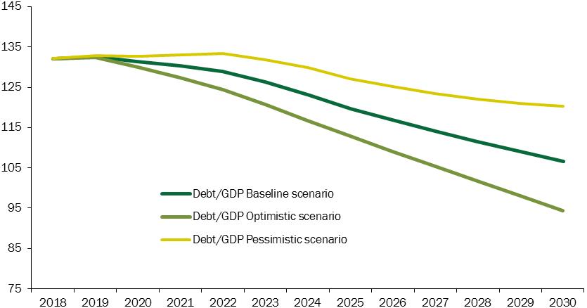
|
|
Source: MEF.
|
IV.3 LONG-TERM SCENARIOS
This
section presents the results of the medium/long-term fiscal
sustainability analysis. The analysis follows the
methodology developed by the EPC-WGA (Economic Policy
Committee - Working Group on Ageing) to update the
projections of expenditure related to the demographic
evolution of the population. The projections use Eurostat’s
demographic projections (with base year 2015) and,
according to certain underlying macroeconomic assumptions
(e.g. labour productivity), also update the GDP and debt-GDP
ratio projections over a reference horizon as far as 2070.
The
update from the previous assessment cycle (2015 to 2017), of
both macroeconomic assumptions and demographic trends, had a
negative impact on the evolution of the long-term labour
factor and GDP growth. Consequently, as already highlighted
in last year's Stability Programme, there has been a marked
deterioration in the ratio of total age-related expenditure
to GDP compared to previous estimates. Nevertheless, the
long-term sustainability of Italy’s public finances is
confirmed.
The impact of ageing on fiscal
sustainability
The
medium-/long-term forecasts of public expenditure on
pensions13, health care, Long-Term
Care (LTC), social safety nets and education for analysing
the
___
13 The forecasts are made on
the assumption that, as already assumed in the public
finance documents, that the early retirement loan program
guaranteed by future pension benefit streams (so-called
market APE) is qualified and classified in the national
accounts as a loan and not as a direct monetary transfer to
households
|
MINISTRY OF
ECONOMY AND FINANCE
|
97
|
|
ECONOMIC
AND FINANCIAL DOCUMENT - SECT. I
STABILITY
PROGRAMME
|
medium to long-term
sustainability of public finances are drawn up in line
with the methodological guidelines defined at European
level under the EPC-WGA. These forecasts include
national accounts data up to 2018 and for the following
four years, the expenditure forecasts included in the
public finance scenario under unchanged legislation. The
scenario assumptions are consistent with the
macroeconomic scenario based on unchanged legislation
prepared for the EFD 2019. In the medium to long term,
the forecast scenarios defined under the EPC-WGA for the
2018 forecast round were adopted, amended to take
account of the impact of the structural pension measures
adopted by Decree Law No. 4/2019 on the stay at work
rates and appropriately linked to the short-term
scenarios14.
The
demographic assumptions are based on the central
scenario developed by Eurostat for 2015. This scenario
envisages for Italy: i) a net flow of immigrants of
around 190,000 average units per year, increasing until
2040 and then falling; ii) life expectancy in 2070 of
86.9 years for men and 90.9 years for women; iii) a
total fertility rate in 2070 of 1.66.
As far
as macroeconomic variables are concerned, the national
accounts data was incorporated for the two-year period
2017-2018. Instead, for the four-year period 2019-2022,
growth assumptions were adopted, both at constant and
current prices, in line with the indications of the
macroeconomic scenario at unchanged legislation of the
EFD 2019. For the following period, the structural
assumptions of the 2018 EPC-WGA baseline scenario were
adopted, amended to reflect the impact on staying in
work of the structural measures adopted by Decree Law
No. 4/2019. These assumptions were
linked, in the transitional phase, with the short-term
dynamics15.
The
long-term dynamics of macroeconomic variables, as
inferred from the assumptions agreed in the EPC WGA
(EPC-WGA baseline 2018 scenario) forecast an average
annual rate of change in real labour productivity that
will increase until 2045, when it stands at around 1.6
percent, before falling to approximately 1.5 percent of
GDP at the end of the forecast period. On the employment
front, the employment rate in the 15-64 age group is
expected to increase from 58.8 percent in 2018 to 62.2
percent in 2070. The interaction of these assumptions
with demographic dynamics determines a growth rate of
real GDP, which, in the period 2023-2070, stands at an
average of around 1 percent per year. Starting from
2025,
and, in the same way, that the provisions of article
23 of Decree Law No. 4/2019 on access to credit for TFS
advances for civil servants are qualified and classified
in the National Accounts as a loan and do not lead to a
reclassification as an advance direct monetary transfer
to households also as a result of the provisions of
article 24 of the same decree.
14 The medium/long-term
scenarios defined for the purposes of preparing the
age-related public expenditure forecasts EPC-WGA 2018
were published in ‘The 2018 Ageing Report: Underlying
Assumptions and Projection Methodologies’ - European
Commission Directorate-General for Economic and
Financial Affairs and provided in advance to the Member
States at the end of May 2017. In relation to the Ageing
Report scenarios, the assumptions underlying the current
projections were amended to take into account the impact
on labour market participation rates of the 9-month
reduction in retirement age due to the block in
adjustments, for the years 2019-2026, for life
expectancy of the contributory retirement age
requirement for the early retirement channel independent
of age, as provided for by Decree Law No. 4/2019. In
relation to the WGA Baseline scenario, the new activity
rates are around 0.1 percentage points lower.
15 The employment
differences highlighted in 2022, when comparing the
EPC-WGA baseline scenario with the short-term
macroeconomic scenario of the 2019 EFD, were
progressively reduced to zero. In particular, both
activity rates and unemployment rates have been
gradually realigned over a five-year period. As regards
productivity dynamics, the assumptions of the EPC-WGA
baseline scenario were substantially confirmed from
2022.
|
98
|
MINISTRY OF ECONOMY AND FINANCE
|
|
IV. SENSITIVITY AND
SUSTAINABILITY OF PUBLIC FINANCES
|
The
forecasts in Table IV.3 are updated on the basis of the
current legislation, including both the measures adopted
by the Budget Law 2019 (Law No. 145/2018) and the social
security measures included in Decree Law No. 4/2019,
implementing the provisions included in the Budget Law16.
In
particular, the projections of pension expenditure take
into account the regulatory measures included in the 2019
Budget Law17 (Law No.
145/2018), including the introduction of the new system of
indexation of pension benefits in force in the period
2019-2021 and the application in the five-year period
2019-2024 of the reduction rate for pensions exceeding
€100,000 gross. Moreover, the projections include all the
effects of the provisions of Decree Law No. 4/2019,
including those deriving from the introduction of the new
early retirement scheme ‘Quota 100’, which, for the period
2019-2021, in the event of the combined requirement of an
age of at least 62 years and no fewer than 38 years of
contributions, allows access to pension benefits even by
combining the non-corresponding insurance periods found in
two or more of the managements indicated by the regulation
and administered by the INPS18.
Finally, the projections of pension expenditure include,
for the early retirement scheme independent of age
requirements and for ‘early-starting’ workers (lavoratori precoci),
the non-application of life expectancy adjustments for the
period 2019-2026. During this interval, regulations allow
access to early retirement regardless of age, having
accrued contributions at least 42 years and 10 months for
men and 41 years and 10 months for women19. For early-starting
workers20, access to pension
benefits is possible once they have accrued at least 41
years' contributions.
As
regards healthcare expenditure, the forecast discounts the
financial effects associated with the postponement to 2019
of the burden for the non-renewal, for 2018 only, of the
agreements for general medical care and for outpatient
medical professionals, as well as the contractual costs,
for the three-year period 2016-2018, for managerial
employees only, following the failure to sign the relevant
contracts, as provided for by the 2018 Budget Law. The
forecast
___
16 The institution of the
Citizens' Income contained in Decree Law No. 4/2019 and
converted into law on 27 March 2019, is not classified as
a social security benefit. In fact, it is a support
welfare service for families in a situation of financial
hardship also aimed at reintegration into the world of
work and social inclusion, and is compatible with income
from work and concurrent redundancy support services. For
this reason, it is not included in the calculation of the
expenditure aggregate considered here, which takes into
account the items relating to pensions, healthcare,
Long-Term Care, redundancy arrangements and education.
17 Paragraph 256 of Budget
Law 145/2018 established the ‘Fund for the revision of the
early retirement system and to encourage the hiring of
young workers’, which has a budget of 7,000 million per
year from 2024. The greater financial burden resulting
from the social security provisions of Decree Law No.
4/2019 was financed by the substantial zeroing of the
expenditure allocation under examination until 2023. In
the following years, under unchanged legislation, the
above-mentioned expenditure authorisation includes
increasing residual amounts reaching around 5 billion euro
per year from 2028. In this context, these residual
allocations, not yet defined by law, are not attributed to
specific structural measures in the field of pensions.
18 The law provides for a
system of starting points (mobile windows), every three
months for private workers and six months for public
workers.
19 The right to start
receiving a pension is finalised three months after
meeting the aforementioned requirements.
20 Even for early-starting
workers, the right to start receiving a pension is
finalised three months after meeting these requirements.
|
MINISTRY OF
ECONOMY AND FINANCE
|
99
|
|
ECONOMIC
AND FINANCIAL DOCUMENT - SECT. I
STABILITY
PROGRAMME
|
also discounts the
costs of renewing contracts and agreements for the
three-year period 2019-2021, in accordance with the 2019
Budget Law21.
With regard to social safety nets, the forecast
also takes into account the progressive effects of
strengthening the protection of social safety nets
provided for by the legislative decrees implementing Law
No. 183/2014 (in particular Legislative Decrees No.
22/2015 and No. 148/2015).
With regard to the education system, the forecast
takes into account the costs of renewing contracts for
the three-year period 2019-2021, pursuant to the 2019
Budget Law, as well as the different methods of funding
the actual workforce, the effects of which are rendered
neutral in the long term.
Table IV.3 includes information on projections
for expenditure for pensions and other social benefits.
According to the new demographic and macroeconomic
assumptions, total age-related expenditure decreases
slightly from 27.9 percent of GDP in 2015 to 27.7
percent in 2020. Subsequently, this expenditure
aggregate gradually increases to reach a peak of 30.9
percent of GDP in 2045. In the final part of the
forecast horizon, the ratio falls again to 27 percent of
GDP in 2070.
With regard to the individual components of
age-related expenditure, after the increase recorded in
previous years, the ratio of pension expenditure to GDP
decreases from 2015 for about three years to reach 15.3
percent in 2018, thanks to a more favourable growth
trend and the gradual continuation of the process of
raising the minimum requirements for retirement.
Subsequently, the ratio resumes growth, reaching 18.4
percent in 2042. In the final phase of the forecast
period, the pension expenditure-to-GDP ratio declines
rapidly to 14.7 percent in 2060 and 13.8 percent in
2070.
As far as healthcare expenditure is concerned,
the forecast was based on the reference scenario
methodology22. In addition to the
effects of demographic ageing, this methodology also
takes into account the effects of additional explanatory
factors that can have a significant impact on the
dynamics of healthcare expenditure. After an initial
reduction as a result of measures to contain expenditure
dynamics, the forecast of the ratio of healthcare
expenditure to GDP increases from 2022 and stands at
around 7.9 percent in 2060 and 7.7 percent of GDP in
2070.
___
21 For further
information, please refer to the detailed analysis found
in Section II of EFD 2019.
22 The reference scenario,
applied from 2023, envisages, in particular, for the
acute component of healthcare expenditure: i) the
‘‘partial’ application of the dynamic equilibrium
methodology, according to which increases in life
expectancy are translated into years lived in good
health at a ratio of 50 percent (instead of 100 percent
as in the case of the ‘full’ application); ii) the
dynamics of the unit cost ‘linked’ to the GDP per
capita; iii) the elasticity of the unit cost with
respect to the GDP per capita higher than the unit (it
decreases line-by-line in the forecast period from the
initial 1.1 to 1 in 2070). For the Long Term Care
component of healthcare expenditure, the reference
scenario envisages: i) the ‘partial’ application of the
dynamic equilibrium methodology, as for the acute
component of healthcare expenditure; ii) the dynamics of
the unit cost ‘linked’ to productivity; iii) the
elasticity of the unit cost to productivity above the
unit (it decreases line-by-line in the forecast period,
going from the initial 1.1 to 1 in 2070).
|
100
|
MINISTRY OF ECONOMY AND FINANCE
|
|
IV. SENSITIVITY
AND SUSTAINABILITY OF PUBLIC FINANCES
|
|
TABLE IV.3 EXPENDITURE FOR PENSIONS,
HEALTHCARE, CARE FOR THE ELDERLY, EDUCATION
AND UNEMPLOYMENT BENEFITS (2010-2070)
|
|||||||||||||
|
|
2010
|
2015
|
2020
|
2025
|
2030
|
2035
|
2040
|
2045
|
2050
|
2055
|
2060
|
2065
|
2070
|
|
Total expenditure
|
49.9
|
50.3
|
49.1
|
49.9
|
51.9
|
54.0
|
55.5
|
56.4
|
56.3
|
55.5
|
55.0
|
54.5
|
54.2
|
|
of which:
|
|||||||||||||
|
- Age-related
expenditure
|
27.5
|
27.9
|
27.7
|
27.6
|
28.7
|
29.8
|
30.7
|
30.9
|
30.1
|
28.9
|
28.1
|
27.5
|
27.0
|
|
Pension
expenditure
|
14.8
|
15.7
|
15.8
|
16.0
|
16.8
|
17.8
|
18.3
|
18.1
|
16.9
|
15.6
|
14.7
|
14.1
|
13.8
|
|
Healthcare expenditure
|
7.1
|
6.7
|
6.6
|
6.6
|
6.9
|
7.1
|
7.4
|
7.6
|
7.8
|
7.8
|
7.9
|
7.8
|
7.7
|
|
of which LTC - health
|
0.8
|
0.7
|
0.7
|
0.7
|
0.7
|
0.8
|
0.9
|
0.9
|
1.0
|
1.1
|
1.1
|
1.1
|
1.1
|
|
LTC -
social/assistance
|
1.0
|
1.0
|
1.0
|
1.1
|
1.1
|
1.2
|
1.2
|
1.3
|
1.5
|
1.6
|
1.6
|
1.6
|
1.6
|
|
Education
expenditure
|
3.9
|
3.6
|
3.5
|
3.3
|
3.2
|
3.1
|
3.1
|
3.3
|
3.3
|
3.4
|
3.4
|
3.3
|
3.4
|
|
Unemployment
benefits
|
0.7
|
0.9
|
0.8
|
0.7
|
0.7
|
0.6
|
0.6
|
0.6
|
0.6
|
0.6
|
0.6
|
0.6
|
0.6
|
|
- Interest
expenditure
|
4.3
|
4.1
|
3.6
|
4.4
|
5.5
|
6.3
|
7.0
|
7.7
|
8.4
|
8.8
|
9.1
|
9.2
|
9.3
|
|
Total Revenue
|
45.6
|
47.7
|
47.0
|
46.8
|
46.8
|
46.8
|
46.8
|
46.7
|
46.7
|
46.7
|
46.7
|
46.7
|
46.7
|
|
of which: Property income
|
0.6
|
0.7
|
0.7
|
0.5
|
0.5
|
0.5
|
0.5
|
0.5
|
0.5
|
0.5
|
0.5
|
0.4
|
0.4
|
|
ASSUMPTION (%)
|
|||||||||||||
|
Labour productivity growth rate
|
2.6
|
0.3
|
0.4
|
0.2
|
0.6
|
0.9
|
1.2
|
1.6
|
1.6
|
1.6
|
1.6
|
1.6
|
1.5
|
|
Real GDP growth rate
|
1.7
|
0.9
|
0.6
|
0.8
|
0.3
|
0.4
|
0.5
|
1.1
|
1.3
|
1.6
|
1.2
|
1.4
|
1.1
|
|
Male participation rate
(20-64) |
78.4
|
79.5
|
80.4
|
80.3
|
80.2
|
80.3
|
80.3
|
80.6
|
80.6
|
80.5
|
80.5
|
80.4
|
80.4
|
|
Female participation rate
(20-64) |
54.6
|
57.8
|
60.7
|
62.6
|
63.7
|
64.2
|
64.5
|
64.6
|
64.7
|
64.7
|
64.7
|
64.7
|
64.8
|
|
Total participation rate (20-64)
|
66.3
|
68.6
|
70.5
|
71.4
|
72
|
72.3
|
72.5
|
72.8
|
72.8
|
72.8
|
72.8
|
72.8
|
72.8
|
|
Unemployment rate
|
8.4
|
11.9
|
11.2
|
9.3
|
8.5
|
8.1
|
7.8
|
7.6
|
7.4
|
7.4
|
7.3
|
7.3
|
7.3
|
|
Population of age 65 and over/ total
population
|
20.4
|
21.7
|
23.1
|
24.7
|
27.1
|
29.8
|
32.1
|
33.5
|
33.8
|
33.7
|
33.4
|
32.9
|
32.8
|
|
Elderly dependency ratio
(65 and over/[20-64]) |
33.6
|
36.4
|
39.1
|
42.5
|
47.9
|
54.8
|
61.8
|
66.3
|
67.7
|
67.5
|
66.6
|
65.4
|
65.4
|
|
Notes: (1) For
the four-year period 2019-2022, growth
assumptions were adopted in line with the
indications of the macroeconomic scenario at
unchanged legislation underlying the EFD 2019.
For the following period, the scenario is
adopted that the EPC-WGA prepared for the
age-related expenditure forecasts for the 2018
round. (2) Until 2018, expenditure on social
benefits refers to National Accounting data.
For the period 2019-2022, the forecast values
are in line with those underlying the forecast
of the public finance scenario. (3) Paragraph
256 of Budget Law No. 145/2018 established the
‘Fund for the revision of the early retirement
system and to encourage the hiring of young
workers’, which has a budget of 7,000 million
per year from 2024. The greater financial
burden resulting from the social security
provisions of Decree Law No. 4/2019 are
financed by the substantial zeroing of the
expenditure allocation under examination until
2023. In the following years, under unchanged
legislation, the above-mentioned expenditure
authorisation includes increasing residual
amounts reaching around 5 billion euro per
year from 2028. In this context, these
residual allocations, not yet defined by law,
are not attributed to specific structural
measures in the field of pensions. (4) The
forecast is based on the reference scenario
methodology. (5) For 2010, the data does not
discount the different accounting of the
interest expense, entirely excluded from the
aggregate of health expenditure for an annual
amount of between 250 and 300 million. (6) The
aggregate includes ISCED levels 1-8 according
to the OECD classification (ISCED 2011 level).
It does not include expenditure for adult
education (lifelong learning) and pre-school
(pre-primary). (7) Rounding up to the first
decimal place may lead to inconsistencies with
the values shown in the table.
Source: MEF
data processing using the Long Term Forecast
Model of the State General Accounting Office.
|
|||||||||||||
The social/assistance component of public
expenditure for long-term care (LTC) consists of
around 4/5 cash benefits and around 1/5 local
social/assistance services23. With regard to the
latter, the expenditure/GDP ratio forecast was based
on the assumptions underlying the reference scenario
as defined for the health component of LTC
expenditure.
___
23 For
more details, see the Ministry of Economy and
Finance-RGS (2018), Report No. 19, chapter 4.
|
MINISTRY
OF ECONOMY AND FINANCE
|
101
|
|
ECONOMIC
AND FINANCIAL DOCUMENT - SECT. I STABILITY PROGRAMME
|
With regard to cash benefits, in
consideration of the specific nature of the
service consisting of monetary amounts paid to the
beneficiary and not the purchase of goods and
services, the amount of the benefits was
structurally ‘linked’ to the dynamics of GDP per
capita from 202324.
After an initial phase of substantial stability,
the social/assistance component of LTC expenditure
presents a growing profile in terms of GDP, which
extends over the entire forecast period, reaching
1.6 in 2070.
The projection of expenditure
for social safety nets in relation to GDP rises
from 0.7 percent in 2010 to 0.9 percent in 2015,
before gradually decreasing and reaching a value
of approximately 0.6 percent from the second half
of the forecast period.
The expenditure projection for
education as a percentage of GDP25 is consistent with
the expenditure aggregate defined in the EPC WGA.
The expenditure-to-GDP ratio shows a gradually
decreasing trend that continues for about fifteen
years. Starting from 2022, this fall is
essentially driven by the drop in student numbers
caused by demographic dynamics. The ratio starts
to grow slightly again in the final part of the
forecast period, reaching around 3.4 percent in
2070.
|
F
O
C
U
S
|
Medium-long term
trends of the Italian pension system
In implementation of
the provisions included in the 2019 Budget
Law (Law No. 145/2018), Decree Law No.
4/201926 has established, on
an experimental basis and only for the
period 2019-2021, a new channel of early
retirement that can be accessed by all
workers who meet the following combined
requirements: age of at least 62 years and
at least 38 years’ accrued contributions.
The law envisages
different rules for retirement for workers
in the private sector and for those in the
public sector. For the former,
postponement is foreseen of the first
effective date of pension benefits of
three months from the date of meeting
these combined requirements. For workers
in the public sector, with the exception
of the school sector, for which specific
provisions apply, access to pension
benefits is finalised 6 months after these
combined requirements have been met27.
Decree Law No. 4/2019 provides for further
measures in the field of pensions. In
particular, the regulations impose a
reduction to the
|
___
24
In line with the methodological indications agreed
in the EPC-WGA for the preparation of the 2018
forecast round, the elasticity of the unit cost
with respect to GDP per capita rises from 1.1 to 1
over the entire forecast period.
25
The definition of education expenditure agreed
within the EPC-WGA includes ISCED levels 1 to 8
according to the 2011 ISCED classification (from 1
to 6 according to the 1997 ISCED classification),
excluding pre-school (pre-primary), which
corresponds to ISCED level 0, and lifelong
learning (See European Commission, Special Report
No. 1/2006). The expenditure aggregate is built on
UNESCO/OECD/EUROSTAT (UOE) data. The forecast
includes UOE data updated to the financial year
2015.
26
Implementing the provisions of Law No. 145/2018
(2019 Budget Law) in terms of related financial
planning. Paragraph 256 of Budget Law No. 145/2018
established the ‘Fund for the revision of the
early retirement system and to encourage the
hiring of young workers’, which has a budget of
7000 million per year from 2024. The greater
financial burden resulting from the social
security provisions of Decree Law No. 4/2019 were
covered by the substantial zeroing of the
allocation of the expenditure authorisation under
examination until 2023. In the following years,
under unchanged legislation, the above-mentioned
expenditure authorisation includes increasing
residual amounts reaching around 5 billion euro
per year from 2028. In this context, these
residual allocations, not yet defined by law, are
not attributed to specific structural measures in
the field of pensions.
27
Pension benefits obtained according to the new
early retirement scheme at least 62 years of age
and with at least 38 years of contributions
cannot be combined, until reaching old-age
retirement age, with income from employment or
self-employment, with the exception of income from
occasional self-employment up to a maximum of
5,000 euro gross per year.
|
102
|
MINISTRY
OF ECONOMY AND FINANCE
|
|
IV. SENSITIVITY AND
SUSTAINABILITY OF PUBLIC FINANCES
|
|
2018 level, i.e. 42
years and 10 months for men and 41 years
and 10 months for women, of the years'
contribution requirement for the channel
of early retirement independent of age
and the freezing, for the period
2019-2026, of the related adjustments to
life expectancy. This channel is also
subject to the system of starting dates,
so that the right to start receiving the
pension is finalised 3 months after
meeting the contributions requirement.
The non-application
of life expectancy adjustments for the
period 2019-2026 is also foreseen for
so-called ‘early-starting’ workers who
are eligible for retirement once they
have accrued at least 41 years'
contributions28. Finally, Decree
Law No. 4/2019 strengthens the ‘Women's
Option’ measure by allowing female
workers who reach 58 years of age by 31
December 2018 for employees and 59 years
for self-employed workers and at least
35 years of contributions to take early
retirement, with the calculation of
retirement benefits29
entirely under the contribution system.
Despite having a
significant financial impact, the new
rules introduced by Decree Law No.
4/2019 have the purpose of making access
to early retirement temporarily easier.
The extension of the
contribution system to all workers,
including those who, according to the
previous legislation, would have
received a pension calculated according
to the wage system (i.e. those who had
more than 18 years of contributions as
at 31/12/1995), is confirmed with effect
from 2012. Moreover, in line with the
regulatory and institutional structures
found in most European countries, the
Italian pension system maintains two
channels of access to retirement30:
(a) an old-age pension with at least 20
years' contributions and a legal age
requirement that, for 2019, is 67 years31;
(b) early retirement, with 20 years'
contributions, allowed up to three years
before the old-age pension age for
workers hired after 1 January 1996 and
subject to reaching a sufficiently high32
level of pension contributions, or
regardless of age and date of
recruitment but with a longer
contribution period.
Starting in 2013, all
age requirements (including those for
access to the social allowance) and
contribution requirements for access to
early retirement, regardless of age, are
indexed to changes in life expectancy as
measured by ISTAT. Aside from that
recently established by Decree Law No.
4/2019, which, for the channel of early
retirement independent of age, requires
the non-application for the period
2019-2026 of the adjustments for life
expectancy; for all the other
requirements for access to retirement,
these adjustments are made every two
years, according to a procedure entirely
administrative in nature33.
|
___
28
Even for early-starting workers, the right to
start receiving a pension is finalised three
months after meeting these requirements.
29
The law also provides for the postponement of
the first effective date of pension benefits by
12 months from meeting the requirements for
female employees and by 18 months for
self-employed women.
30
Safeguard measures have also been envisaged to
ensure a more gradual implementation of the 2011
reform, i.e. taking account of specific details
in relation to the proximity to retirement and
difficult situations related to staying in the
labour market, cases which have all been
specifically identified at regulatory level.
31
In addition, for workers recruited after 1
January 1996, for whom the pension is fully
calculated using the contributions system,
access to old-age retirement is also subject
reaching a minimum pension amount of 1.5 times
the 2012 social allowance revalued on the basis
of GDP trends.
32
For these workers, for whom the pension is fully
calculated using the contribution system, access
to early retirement is also subject to achieving
a minimum pension amount of 2.8 times the social
allowance revalued on the basis of GDP trends.
33The
adjustment of the requirements starting in 2016
(4 additional months), in compliance with the
provisions of the law (article 12, paragraph
12-bis, of Decree Law No. 78 of 31 May 2010,
converted with amendments by Law No. 122 of 30
July 2010), was adopted at least twelve months
before the start of the adjustment by
Directorial Decree of 16 December 2014,
published in the Official Journal on 30 December
2014, and that of the conversion coefficients by
Directorial Decree of 22 June 2015, published in
the Official Journal on 6 July 2015. The
adjustment of the requirements starting in 2019
(additional 5 months), in compliance with the
provisions of the law, was adopted at least
twelve months before the adjustment started with
Directorial Decree dated 5 December 2017,
published in the Official Journal on 12 December
2017. The current legislation provides for a
guarantee clause according to which the minimum
old-age requirement may not be less than 67
years for
|
MINISTRY OF ECONOMY AND
FINANCE
|
103
|
|
ECONOMIC
AND FINANCIAL DOCUMENT - SECT. I STABILITY
PROGRAMME
|
|
Moreover, from
2013, the calculation of the
conversion coefficients34 at the time of
retirement was extended to the
old-age requirement age plus four
years.
According to this
regulatory framework, the figure
below shows the forecast of pension
expenditure as a percentage of GDP
at unchanged legislation35, based on the
EPC-WGA Baseline scenario36.
|
|
FIGURE R.1: PUBLIC
EXPENDITURE FOR PENSIONS AS A
PERCENTAGE OF GDP
|
|
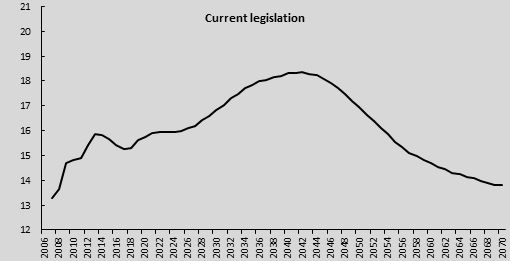 |
|
|
Notes: The EPC-WGA Baseline
scenario incorporates, in the short
term, the general trends indicated
in the 2019 Stability Programme.
Source:
Long Term Forecast Model of the
State General Accounting Office.
|
|
After the growth
recorded between 2008 and 2014,
exclusively due to the continuation
of the recessionary phases of the
economic cycle, from 2015, thanks to
the more favourable economic growth
and to the gradual continuation of
the process of raising the minimum
retirement requirements and the
pro-rata application of the
contribution calculation system, the
ratio of pension expenditure to GDP
decreases for around three years.
Subsequently, the ratio of pension
expenditure to GDP begins a long
period of growth that lasts until
2042, reaching a peak of 18.4
percent. In the first phase, this
increase is explained in part by the
slowdown in the dynamics of
short-term gross domestic product
and that assumed in the
|
those who are eligible for retirement as of the first effective date from 2021. In any case, according to ISTAT's demographic forecasts, the aforementioned objective could be assured as early as 2019.
34
The conversion factor is also adjusted in
accordance with the same timetable as for
the adjustment of the eligibility
requirements for retirement. The adjustment,
effective from 1 January 2016, was adopted
by Directorial Decree of 22/06/2015,
published in Official Journal No. 154 of 6
July 2015, while the adjustment of 2019 was
approved by Directorial Decree of 15 May
2018, published in Official Journal No. 131
of 8 June 2018.
35
The forecasts are elaborated on the
assumption that the institution of the
pension guarantee financial advance
(so-called market APE) is qualified and
classified in the national accounts as a
loan and not as a direct monetary transfer
to households and, in the same way, that the
provisions of article 23 of Decree Law No.
4/2019 on access to credit for advance TFS
for civil servants are qualified and
classified in the National Accounts as a
loan and do not involve a reclassification
as an advance of direct monetary transfer to
households also as a result of the
provisions of article 24 of the same decree.
36
The pension expenditure forecasts as a ratio
of GDP take into account, for the four-year
period 2019-2022, the growth assumptions,
both at constant prices and at current
prices, of the short-term macroeconomic
scenario at unchanged legislation defined
for the EFD 2019. For the following period,
the structural assumptions of the 2018
EPC-WGA baseline scenario were adopted,
amended to reflect the impact of the
structural measures adopted by Decree Law
No. 4/2019 on time at work.
|
104
|
MINISTRY
OF ECONOMY AND FINANCE
|
|
IV. SENSITIVITY
AND SUSTAINABILITY OF PUBLIC
FINANCES
|
|
EPC-WGA Baseline37
scenario and, in part, by greater
recourse to retirement, because of the
measures provided for by Decree Law
No. 4/2019. In a second phase, after
2030, the growth in the ratio between
pension expenditure and GDP is
attributable to the increase in the
number of pensions compared to the
number of employees due to the
retirement of the baby boom
generations, which is only partly
offset by the increase in the minimum
pension requirements and by the effect
of limiting the pension amounts
exerted by the gradual application of
the system for calculating
contributions over the entire working
life.
After the peak in
2042, the ratio of pension expenditure
to GDP falls rapidly to 16.9 percent
in 2050 and 14.7 percent in 2060,
converging to 13.8 percent in 2070,
with an almost constant deceleration
over the entire period. The rapid
reduction in the ratio between pension
expenditure and GDP in the final phase
of the forecast period is due to the
generalised application of the
contribution calculation, which is
accompanied by the stabilisation and
subsequent trend reversal of the ratio
between the number of pensions and the
number of people in employment.
This trend is
explained both by the gradual exit of
the baby-boom generations and by the
automatic adjustment of the minimum
retirement requirements according to
life expectancy.
The figure below
presents the forecast of pension
expenditure as a share of GDP under
unchanged legislation and compares it
with that which would have occurred as
a result of the schemes preceding the
main reform measures. Compared to the
immediately preceding legislation, in
the period 2019-2036, the measures
found in Decree Law No. 4/2019 and in
the Budget Law for 2019 (Law No.
145/2018) included in the scenario at
unchanged legislation generate an
increase in the incidence of pension
expenditure as a percentage of GDP
equal of an average 0.2 points per
year, progressively decreasing from
the first years of the forecast, where
there is a greater incidence of
expenditure as a percentage of GDP. In
the long term, thanks to the overall
reform process implemented from 2004,
the average retirement age (taking
into account both the old-age
retirement age and the requirements
for early retirement) increases from
60-61 during the period 2006-2010 to
about 63 in 2017, 67 in 2040 and then
about 68 in 2050. Cumulatively, the
lower expenditure to GDP ratio
resulting from the overall reform
process launched in 2004 amounts to
around 60 percentage points of GDP by
2060.
|
___
37
As already outlined in the Update Note to the
2017 EFD, in the 2018 EFD (Section I, 2018
Stability Programme) and in the 2018 Update
Note to the 2018 EFD, the EPC-WGA Baseline
scenario prepared for the 2018 forecast round
showed significant deterioration in Italy
compared to the previous one (2015 round),
attributable to the revision of the
demographic scenario by Eurostat and of the
medium-term macroeconomic scenario by the
European Commission.
|
MINISTRY OF ECONOMY AND
FINANCE
|
105
|
|
ECONOMIC
AND FINANCIAL DOCUMENT - SECT. I STABILITY
PROGRAMME
|
|
FIGURE R.2: PUBLIC
EXPENDITURE FOR PENSIONS AS A
PERCENTAGE OF GDP UNDER DIFFERENT
REGULATORY ASSUMPTIONS
|
|
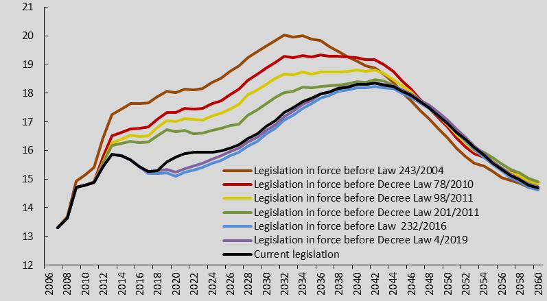
|
|
|
Notes: The EPC-WGA Baseline
scenario incorporates, in the short
term, the general trends indicated
in the 2019 Stability Programme.
Source: Long Term Forecast
Model of the State General
Accounting Office.
|
Long-term debt dynamics
and fiscal sustainability indexes
The use of
age-related expenditure and GDP projections
over the long term, together with additional
public finance assumptions, makes it
possible, again in accordance with the
fiscal surveillance methodology used by the
European Commission, to obtain debt
forecasts until 2070. Following this
approach, tax revenues are assumed constant
in relation to GDP, at the 2022 level,
throughout the forecast period. Public
expenditure, on the other hand, as already
mentioned, varies according to the
population dynamics. Finally, the GDP
deflator converges to 2.0 percent from 2023
and the real interest rate, starting from
the 2022 level, converges to 3.0 percent in
ten years38.
As shown
in Figure IV.7, the long-term forecasts of
debt-to-GDP in the reference scenario of
this document outline a growing trend, with
debt forecast to be around 193.1 percent of
GDP in 2070. This is worse than the national
scenario forecasts, which predict a
debt-to-GDP ratio of 113.8 percent in 207039.
___
38
European Commission, 2017, The 2018 Ageing
Report: Underlying assumptions and
Projection Methodologies, European Economy,
Institutional Papers, No. 65
(https://ec.europa.eu/info/sites/info/files/economy-finance/ip065_en.pdf).
39
The long-term projections for the national
scenario are based, for the demographic
assumptions, on the ISTAT median scenario
for 2017. This scenario envisages: i) an
annual net flow of immigrants of an average
165,000 units; ii) life expectancy in 2070
of 86.5 years for men and 90.6 years for
women; iii) a total fertility rate in 2070
of 1.61. With regard to macroeconomic
variables, for the two-year period
2016-2017, the national accounting data has
been incorporated, and for the four-year
period 2019-2022, the growth forecasts of
the overall macroeconomic trends of the EFD
2019 were adopted, at both constant and
current prices. For the subsequent period,
the macroeconomic trends of the national
scenario discounts the productivity growth
rate
|
106
|
MINISTRY OF ECONOMY AND
FINANCE
|
|
IV.
SENSITIVITY AND
SUSTAINABILITY OF PUBLIC
FINANCES
|
Comparison
between the national scenario and the
EFD 2019 scenario reveals a different
debt trend, deriving from the
demographic assumptions underlying the
estimated evolution of public spending
and economic growth. As has been pointed
out on several occasions, the update of
the demographic scenario under the
EPC-AWG, together with the revision of
the macroeconomic assumptions,
contributed significantly to changing
the expected dynamics of the debt/GDP
ratio.
|
FIGURE IV.7: DEBT-TO-GDP
RATIO: COMPARISON OF PROJECTION
SCENARIOS
|
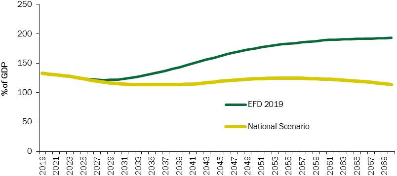
|
|
Source:
MEF analysis based on the Long
Term Forecast Model of the State
General Accounting Office.
|
The baseline scenario is also
used to calculate the medium and
long-term indexes (S1 and S2) used by
the European Commission to estimate the
adjustment needed to achieve fiscal
sustainability, also taking into account
the impact of implicit liabilities
related to population ageing. In
particular, the medium-term S1 index
measures the adjustment of the
structural primary balance to be
achieved in cumulative terms over the
five years following the last year of
the forecast, so as to ensure, if kept
constant in subsequent years, that a 60
percent debt-to-GDP ratio is reached
within fifteen years and that the higher
age-related costs are also financed. As
a result of its construction, the
parameters of the S1 index are
established with respect to the public
debt target set out in the Stability and
Growth Pact. The long-term S2
sustainability index, on the other hand,
shows the fiscal adjustment in terms of
the structural primary balance, which,
if achieved and maintained from the last
year of the forecast onwards, would
maintain the interim balance of the
budget over an infinite period of time.
In
the Commission's interpretation, the
higher and more positive the values of
the S1 and S2 sustainability indexes,
the greater the fiscal adjustment
required to achieve the objective of
debt sustainability and therefore the
risk of fiscal
that
gradually increases from 0.4 percent in
2020 to a peak of 1.6 percent in 2045
and then falls to 1.5 percent in the
final part of the forecast period. The
activity rate in the 20-64 age group
increases from 68.6 percent in 2015 to
76 percent in 2070, while, at the end of
the forecast period, the unemployment
rate converges to 5.5 percent. According
to these demographic and macroeconomic
assumptions, the growth rate of real GDP
is around 1.2 percent per year on
average in the long term, with an
increasing trend in the first decade,
decreasing in the following twenty years
and recovering slightly in the final
part of the forecast period. For further
details, see RGS, 2018, Report on
Medium-Long-Term Trends in the Pension,
Social Care and Healthcare System, No.
19.
|
MINISTRY OF ECONOMY
AND FINANCE
|
107
|
|
ECONOMIC AND
FINANCIAL DOCUMENT -
SECT. I
STABILITY
PROGRAMME
|
sustainability.
Ultimately, the fiscal risk reflects
the initial structural primary
balance, the value of current debt
and the projected dynamics of
age-related public expenditure
costs. Both indexes are based on the
projected growth and budget balances
of the EFD 2019 and incorporate
medium to long-term forecasts of
age-related expenditure.
Table
IV.5 shows the results of the S1 and
S2 indexes and their respective
components estimated by the Ministry
of Economy and Finance in the latest
Stability Programmes and by the
European Commission in the Fiscal
Sustainability Report40 and the Debt
Sustainability Monitor41.
The
value of the S1 index estimated by
the Ministry of the Economy and
Finance shows a deterioration
compared to previous documents,
largely due to the updating of
demographic projections and the
revision of macroeconomic
assumptions. The breakdown of S1 by
sub-component shows that the
adjustment needed to stabilise the
debt-to-GDP ratio at the current
level is -0.8 GDP points, which
almost offsets the component related
to the costs of population ageing.
The component that most affects the
index is the adjustment needed to
reduce the debt ratio from its
initial level to 60 percent of GDP
in 2034. This component assumes a
cumulative fiscal adjustment over
the five-year period 2022 - 2026 of
5.1 p.p. of GDP. The overall value
of the index is 6.1 p.p. of GDP,
higher than the medium-term high
risk threshold set by the European
methodology at 2.5 p.p. of GDP.
The
S1 index estimated by the European
Commission and presented in the
Fiscal Sustainability Report 2018
differs from the index estimated by
the Ministry of the Economy and
Finance mainly for the different and
more unfavourable forecasts of
public finance and underlying
macroeconomic conditions42. It should be
noted that the public finance
forecast starts from the last year
of the time horizon, which for the
MEF is 2022, whereas for the
Commission it is 2020. In the
analysis of the Commission, the
initial structural primary surplus
is 0.4 percent of GDP; in the same
year, the Ministry of the Economy
and Finance estimates a structural
primary surplus of 2.2 percent of
GDP. Given these considerations,
according to the Commission's
estimates, it would be necessary to
achieve a cumulative structural
primary surplus over the period
2021-2025 of 9.4 percentage points
of GDP, i.e. an average annual
consolidation of around 2 p.p. of
GDP, in order to lower the
debt-to-GDP ratio to 60 percent in
2033. The adjustment cost is due for
4.9 p.p. to the distance between the
current debt-to-GDP ratio and the
target to be achieved, for 2 p.p. to
the stabilisation of the debt-to-GDP
ratio given the initial fiscal
position and for 1.6 p.p. to the
additional cost due delays in fiscal
adjustment. The higher expenditure
related to demographic dynamics
represents around 0.9 p.p. of GDP.
___
40 European
Commission, 2019, Fiscal
Sustainability Report 2018,
Institutional Papers 094. January
2019, available at: https://ec.europa.eu/info/publications/economy-finance/fiscal-sustainability-report-2018_en
41 European
Commission, 2019, Debt
Sustainability Monitor 2017,
Institutional Papers 071. January
2018, available at: https://ec.europa.eu/info/sites/info/files/economy-finance/ip071_en.pdf
42 S1 estimates
also differ over a different time
horizon: the debt/GDP target of 60
percent must be achieved over
fifteen years, with 2019 as the base
year, while in this document the
base year is 2019. In addition, the
Commission adopts forecasts with no
policy changes, while the EFD uses
the policy scenario.
|
108
|
MINISTRY
OF ECONOMY AND FINANCE
|
|
IV. SENSITIVITY AND
SUSTAINABILITY OF PUBLIC
FINANCES
|
|
TABLE
IV.4: SUSTAINABILITY
INDICATORS (points of GDP)
|
|||||||
|
|
EFD
2019
|
2018
Fiscal Sustainability
Report
|
EFD
2018
|
Debt
Sustainability Monitor
2017
|
EFD
2017
|
2015
Fiscal Sustainability
Report
|
EFD
2016
|
|
S1
Index
|
|||||||
|
Total
adjustment
|
6.1
|
9.4
|
6.4
|
6.7
|
3.9
|
4.2
|
3.9
|
|
of which:
|
|||||||
|
For
debt/GDP ratio
stabilisation
|
-0.8
|
2.0
|
-1.6
|
0.4
|
-2.8
|
-1.4
|
-2.8
|
|
For the
adjustment delay
|
1.1
|
1.6
|
1.3
|
1.1
|
0.7
|
0.7
|
0.7
|
|
To reach
the 60% target
|
5.1
|
4.9
|
5.6
|
5.1
|
5.6
|
5.1
|
5.6
|
|
For
ageing costs
|
0.8
|
0.9
|
1.0
|
0.1
|
0.3
|
-0.2
|
0.3
|
|
S2
Index
|
|||||||
|
Total
adjustment
|
0.2
|
2.9
|
0.2
|
0.6
|
-1.9
|
-0.9
|
-1.9
|
|
of which:
|
|||||||
|
For
debt/GDP ratio
stabilisation
|
-0.6
|
1.8
|
-1.3
|
0.5
|
-2.0
|
-0.8
|
-2.0
|
|
For
ageing costs
|
0.8
|
1.1
|
1.5
|
0.1
|
0.1
|
-0.1
|
0.1
|
|
Source:
MEF data analysis.
|
|||||||
In
the long term, on the other hand,
Italy confirms its ability to meet
its debt obligations. In fact, the
S2 index used in European fiscal
surveillance, both in the Ministry
of the Economy and Finance's and
the Commission's estimates, is far
from the critical high-risk
threshold (characterised by the
necessary fiscal consolidation of
6 p.p. of GDP). The overall value
of the S2 index estimated by the
Ministry of the Economy and
Finance is 0.2 percent, which is
below the threshold of 2 p.p. of
GDP, under which a country is
considered to be at low risk in
the long term. This value is due
to the higher costs linked to
population ageing. On the other
hand, the value of the component
that measures the adjustment
needed to stabilise the
debt-to-GDP ratio at the 2022
level is -0.6 GDP points. In the
Fiscal Sustainability Report 2018,
the European Commission estimates
a cumulative fiscal consolidation
of 2.9 p.p. of GDP of the
structural primary balance
necessary to stabilise the
debt-to-GDP ratio over the long
term and under unchanged policy
conditions43.
Sensitivity analysis of
long-term debt dynamics
In
order to test the strength of the
long-term debt-to-GDP ratio
forecast in the baseline scenario
against its characteristic
uncertainty, certain sensitivity
scenarios are constructed to
measure the debt-to-GDP ratio's
response to demographic,
macroeconomic and fiscal shocks.
The following scenarios therefore
replicate the assumptions
underlying the sensitivity
exercises presented in the last
2018 Ageing Report by the European
Commission.
___
43 From this
edition, the Fiscal Sustainability
Report 2018 bases the assessment
of long-term fiscal sustainability
on the joint use of debt
sustainability analysis (DSA) and
the S2 index. Overall, Italy is
now at high risk; in fact, the S2
index indicates a medium risk
level (not lower, as in the 2015
Fiscal Sustainability Report)
while the DSA indicates a high
risk.
|
MINISTRY
OF ECONOMY AND FINANCE
|
109
|
|
ECONOMIC AND
FINANCIAL DOCUMENT -
SECT. I STABILITY
PROGRAMME
|
Simulations
with regard to demographic
variables
Population ageing and
migratory flows are among the
most critical issues that Italy
will have to face in the coming
decades. In this regard, it is
particularly important to assess
the impact of the main
determinants of demographic
change separately, namely: i)
the increase in life expectancy;
ii) the trend in the fertility
rate of the population and iii)
the net flow of immigration.
These factors have an impact on
public spending and hence on the
evolution of debt in the long
run.
Figure IV.8 shows the
long-term evolution of debt
following the alteration of the
assumptions on demographic
variables of fertility and
longevity. As already mentioned,
the demographic assumptions of
the EPC-AWG scenario envisage
the following for Italy: i) a
level of life expectancy in 2070
of 86.9 years for men and 90.9
years for women; ii) a total
fertility rate in 2070 of 1.66.
Assuming a deviation from the
baseline scenario due to the
progressive reduction in the
fertility rate of 20 percent
from 2019 onwards, the effect
observed is an increase in the
debt-to-GDP ratio, which is an
average 2.9 GDP points for the
projection horizon 2023-2070,
increasing at the end of the
period. In a scenario that
discounts the assumptions of a
progressive increase in life
expectancy at birth of around 2
years higher in 2070 than in the
reference scenario, the
debt-to-GDP ratio decreases, in
the period 2023-2070, by an
average 6.6 points of GDP
compared to the baseline
scenario.
|
FIGURE
IV.8: SENSITIVITY OF
PUBLIC DEBT TO A RISE IN
LIFE EXPECTANCY AND A
REDUCTION IN THE
FERTILITY RATE (as a
percentage of GDP)
|
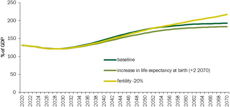 |
|
Source:
MEF analysis based on
the Long Term Forecast
Model of the State
General Accounting
Office.
|
In line with the
assumptions agreed under the
EPC-AWG and according to a
demographic scenario developed
ad hoc by Eurostat, the net flow
of immigrants is around 190,000
annual average units, increasing
to 2040 and decreasing
thereafter. The sensitivity
exercise assumes two alternative
scenarios for the period
2023-2070: i) a 33 percent
decrease in the average net
annual flow of immigrants
compared to the base
assumptions, starting in 2019;
ii) a 33 percent increase in the
net flow of immigrants, again
starting in 2019. The evolution
of public debt in the two
alternative scenarios is
compared with that of the
|
110
|
MINISTRY
OF ECONOMY AND FINANCE
|
|
IV. SENSITIVITY
AND SUSTAINABILITY OF
PUBLIC FINANCES
|
reference
scenario in Figure IV.9. With
the same structural primary
balance as in 2022 and given
the initial debt, an increase
in net migration flows of 33
percent from 2019 would allow
the debt-to-GDP ratio to be
significantly reduced with
respect to the baseline, with
an average reduction of around
18.5 GDP points over the
period 2023-2070.
|
FIGURE
IV.9: SENSITIVITY OF
PUBLIC DEBT TO AN
INCREASE/REDUCTION OF
THE NET FLOW OF
IMMIGRANTS (as a
percentage of GDP)
|
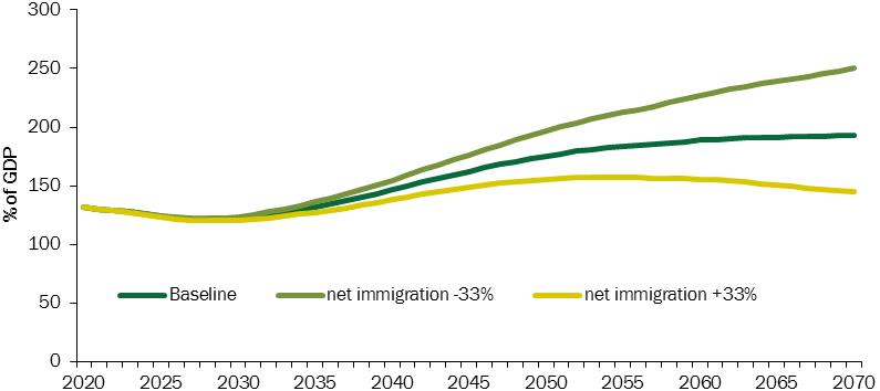
|
|
Source:
MEF analysis based on
the Long Term Forecast
Model of the State
General Accounting
Office.
|
On the other hand, the
decrease in net migration
flows from 2019 would have the
effect of increasing debt,
with an average increase over
the baseline of around 20.5
GDP points from 2023 to 2070.
Simulations
with regard to macroeconomic
variables
The sensitivity
analysis of macroeconomic
variables aims to test the
strength of the debt-to-GDP
ratio forecasts against
alternative assumptions on
more or less favourable
dynamics of Total Factor
Productivity (TFP) and total
employment rate.
With regard to TFP, the
simulation exercise envisages
two alternative scenarios in
which it is assumed that TFP
growth is, respectively, 0.4
percentage points higher or
lower (gradually from 2026 and
standard from 2045) than in
the baseline scenario. In the
baseline scenario, labour
productivity growth for 2020
is estimated at 0.5 percentage
points, rising to 1.6
percentage points in 2045. The
impact on sustainability of a
greater (worse) TFP dynamic is
quite small in the short and
medium term but becomes
substantial over a longer
horizon (Figure IV.10). In the
event of low TFP growth, the
debt-to-GDP ratio would be
higher than the baseline by an
average 29.6 percent of GDP in
the period 2023-2070, while in
the event of high TFP growth,
the debt would reduce by an
average 25.1 percent of GDP
vis-à-vis the baseline
scenario.
|
MINISTRY
OF ECONOMY AND
FINANCE
|
111
|
|
ECONOMIC
AND FINANCIAL
DOCUMENT - SECT.
I STABILITY
PROGRAMME
|
|
FIGURE
IV.10: SENSITIVITY
OF PUBLIC DEBT TO
MACROECONOMIC
ASSUMPTIONS, HIGHER
AND LOWER GROWTH OF
TOTAL FACTOR
PRODUCTIVITY (as a
percentage of GDP)
|
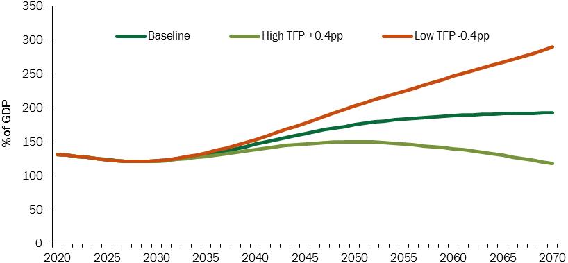
|
|
Source:
MEF analysis based
on the Long Term
Forecast Model of
the State General
Accounting Office.
|
Another
simulation scenario assumes
that the employment rate,
calculated on the 20-64
population, will
increase/decrease gradually
from 2019 onwards, compared
to the baseline assumption,
to 2 percentage points in
2030, and remain at this
level for the remainder of
the period. In the event of
a decrease in the employment
rate, the debt-to-GDP ratio
dynamics would be around
11.2 percent of GDP higher
than the baseline for the
period 2023-2070, while, at
the same time, an increase
would reduce the debt-to-GDP
ratio by an average 11.3
percent of GDP compared to
the baseline (Figure IV.11).
|
FIGURE
IV.11: SENSITIVITY
OF PUBLIC DEBT TO
MACROECONOMIC
ASSUMPTIONS,
EMPLOYMENT RATE (as
a percentage of GDP)
|
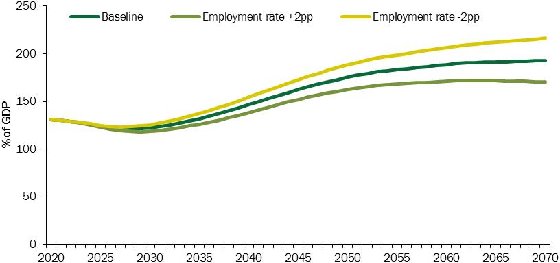
|
|
Source:
MEF analysis based
on the Long Term
Forecast Model of
the State General
Accounting Office.
|
|
112
|
MINISTRY
OF ECONOMY AND
FINANCE
|
|
IV.
SENSITIVITY AND
SUSTAINABILITY
OF PUBLIC
FINANCES
|
Simulations
with regard to the primary
surplus
This
simulation assesses the
strength of the public
finance sustainability
results against a
deterioration in the
primary surplus in 2022.
To this end, the value of
the primary surplus in the
baseline scenario of this
Economic and Financial
Document, equal to 2.3
percent of GDP in 2022, is
reduced by 1 and 2 GDP
points, falling to 1.3 and
0.3 percent respectively
(Figure IV.12).
|
FIGURE
IV.12: SENSITIVITY
OF PUBLIC DEBT TO
THE PRIMARY
SURPLUS (as a
percentage of GDP)
|
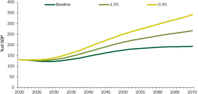
|
|
Source:
MEF analysis based
on the Long Term
Forecast Model of
the State General
Accounting Office.
|
Public
debt dynamics change
significantly because of
the deterioration of the
primary surplus in 2022.
In fact, it should be
noted that, for an initial
primary surplus reduced by
1 percentage point of GDP,
public debt is around 33.2
points higher than the
baseline in the period
2023-2070. If the event
that the primary surplus
in 2022 is permanently
reduced by 2 GDP points
compared to the baseline,
the debt-to-GDP ratio
increases on average by
about 66.8 points over the
period 2023-2070.
Simulations
with regard to pension
reforms
This
section presents a
prospective assessment of
the financial effects of
the intense season of
social security reforms in
the last two decades.
These reforms have
contributed significantly
to reducing the projected
costs of population
ageing.
In this
regard, Figure IV.13
describes the effect on
the debt-to-GDP ratio of
the various legislative
measures adopted from 2004
until the last
intervention approved by
Decree Law No. 4/2019 by
virtue of a counterfactual
exercise that recalculates
the initial debt and
primary surplus in the
absence of the pension
reform in question.
|
MINISTRY
OF ECONOMY AND
FINANCE
|
113
|
|
ECONOMIC
AND FINANCIAL
DOCUMENT -
SECT. I STABILITY
PROGRAMME
|
|
FIGURE
IV.13: IMPACT OF
THE REFORMS ON
THE DEBT-TO-GDP
RATIO (as a
percentage of
GDP)
|
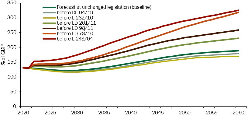 |
|
Source: MEF analysis based on the Long Term Forecast Model of the State General Accounting Office.
|
Excluding
the measures approved at
the beginning of 2019
and at the end of 2016,
which involved a slight
upward revision of the
long-term debt
projections, all
previous reform
measures, from 2004
onwards, have clearly
reduced the ratio of
pension expenditure to
GDP compared to the
projections of previous
legislation, thus
affecting the current
expected expenditure
flows (see Focus
‘Medium/long-term trends
of the Italian pension
system’).
The
results show that, in
the scenario discounting
the absence of the
reforms adopted since
2004, the debt-to-GDP
ratio would increase
substantially over the
entire forecast period,
reaching levels higher
than those of the
reference scenario,
which instead
incorporates the effects
of all the reforms
subsequently
implemented.
|
F
O
C
U
S |
Guarantees
granted by the
State
As at 31 December 2018, the stock of guarantees granted by the State had reached 74.4 billion, or 4.2 percent of GDP. The increase of approximately 6.5 billion compared to the previous year is mainly due to the increase in GACS (+6.3
billion) and
guarantees for
non-market risks
in favour of
SACE (+5.8
billion). The
increase was
also due to the
guarantees
relating to bond
issues by Cassa
Depositi e
Prestiti
S.p.A. and
guarantees in
favour of
households for
first homes and
small and
medium-sized
enterprises,
which increased
by a total of
7.3 billion
compared to
2017. Overall,
guarantees
granted to
financial sector
institutions,
including banks,
GACS and those
relating to Cassa
Depositi e
Prestiti,
amounted to
approximately 21
billion (1.2
percent of GDP),
down by 4.2
billion compared
to 2017. In
particular, the
absence of
guarantees in
favour of
Italian banks
(-12.5 billion)
more than offset
the increase in
GACS.
|
|
TABLE
R.1: PUBLIC
GUARANTEES (in
millions)
|
|||
|
2018
|
|||
|
Level
|
As a % of
GDP
|
||
|
Guarantee
stock
|
74,379
|
4.2
|
|
|
of
which: financial
sector
|
20,850
|
1.2
|
|
|
114
|
MINISTRY
OF ECONOMY AND
FINANCE
|
|
IV.
SENSITIVITY
AND
SUSTAINABILITY
OF PUBLIC
FINANCES
|
|
The
following
components
contributed to
the total
amount:
•
Central
Guarantee Fund
for small and
medium-sized
enterprises.
This is an
industrial
policy
instrument of
the Ministry
of Economic
Development
that benefits
from the State
guarantee and
operates
through three
distinct
actions:
direct
guarantee,granted
to banks and
financial
intermediaries;
reinsurance/counter-guarantee
for guarantees
awarded by
Confidi and
other
guarantee
funds;
co-guarantee
granted
directly in
favour of the
financing
subjects and
jointly with
Confidi and
other
guarantee
funds or
guarantee
funds
established
within the EU
or co-financed
by it. It has
taken on a
central role
in
counter-cyclical
economic
policy
measures. As
at 31 December
2018, the
residual debt
guaranteed
amounts to
approximately
25,735
million.
•
TAV
S.p.A.
The Ministry
of Economy and
Finance
guarantees
that Ferrovie
dello Stato
S.p.A. will
fulfil its
obligations
towards TAV
S.p.A. in
relation to
the
concession,
construction
and management
of the High
Speed system.
This is a
guarantee
aimed at
securing the
financial
resources from
the market
needed to
build the
high-speed
network. As at
31 December
2018 the
residual debt
guaranteed
amounted to
approximately
1,352 million.
•
GACS
(Guarantee on
the
securitisation
of
non-performing
loans).
This is a tool
that the
Treasury makes
available to
credit and
finance
operators to
facilitate the
disposal of
non-performing
bank loans.
The State only
guarantees the
senior
segments of
the
securitised
Non Performing
Loans
portfolios,
i.e. the
safest ones,
which
ultimately
bear any
losses arising
from
sub-expected
loan
recoveries:
the riskiest
segments
cannot be
repaid unless
the senior
tranches
guaranteed by
the State have
been repaid in
full in
advance. The
price of the
guarantee is
market-based,
as also
recognised by
the European
Commission,
which agrees
that the
scheme does
not provide
for State aid
that could be
detrimental to
competition.
As at 31
December 2018,
the residual
debt
guaranteed is
7,734 million.
•
Guarantees
provided by
local
authorities.
The data
relating to
guarantees
granted by
local
authorities
are provided
by the Bank of
Italy, which
collects them
through the
information
transmitted,
by means of
supervisory
reports,
directly from
the financial
institutions
that benefit
from them. As
at 31 December
2018 the
residual debt
guaranteed
amounted to
approximately
2,750 million.
•
Italian
banks.
These
guarantees are
granted by the
State on the
Italian banks’
liabilities in
relation to
bonds issued
by credit
institutions.
As at 31
December 2018,
the residual
debt
guaranteed
amounted to
approximately
8,616 million.
•
Bond
issues by
Cassa Depositi
e Prestiti
S.p.A..
By Decree of
the Minister
of the Economy
and Finance
No. 2545027 of
24 December
2015, a State
guarantee was
granted on the
bond issues of
Cassa
Depositi e
Prestiti
S.p.A. for a
maximum amount
of 5 billion,
in order to
ensure that
the resources
were raised
for the
performance of
public
financing
activities. As
at 31 December
2018,
guarantees
were granted
for a total of
4,500 million.
•
Guarantee
fund for first
homes
(art. 1,
paragraph 48,
letter c of
the Stability
Law 2014),
which
guarantees 50
percent of
mortgage loans
for the
purchase,
renovation and
energy
efficiency
improvements
of buildings
used as main
residence. In
2018, compared
to 46,784 new
loans granted
by the banking
system for a
total of 5,230
million, new
guarantees
were granted
for
approximately
2,615 million,
thus the
guarantees
outstanding
amount to
4,348 million.
•
Guarantee
for non-market
risks in
favour of
SACE.
The State
reinsures,
upon
consideration,
part of the
non-market
risks already
assumed by
SACE S.p.A.
for
transactions
involving
strategic
sectors of the
Italian
economy or
companies of
significant
national
interest in
terms of
employment
levels,
turnover or
repercussions
for the
national
productive
economic
system, which
determine high
concentration
risks for SACE
towards
individual
counterparties,
groups of
connected
counterparties
or destination
countries and
amount to
18,944
million. The
estimate is
preliminary
insofar as it
is based on
data available
as at 30
September
2018.
|
|
MINISTRY
OF ECONOMY AND
FINANCE
|
115
|
|
ECONOMIC
AND FINANCIAL
DOCUMENT -
SECT. I STABILITY
PROGRAMME
|
|
•
State
guarantees in
favour of
ILVA. The
guarantees are
granted on
loans of up to
400 million
issued by the
banking system
in favour of
the
commissioner
of ILVA
S.p.A., in
order to
perform the
investments
necessary for
environmental
remediation,
as well as
those intended
for research,
development
and
innovation,
training and
employment. As
at 31 December
2018,
guarantees
were granted
for a total of
400 million.
In
comparison
with its main
European
partners, in
2017 Italy was
confirmed as
one of the
countries with
the lowest
level of
public
guarantees.
The stock of
guarantees, as
in most EU
countries, is
smaller than
observed in
the two years
following the
financial
crisis of
2011, due to
the
progressive
reduction of
guarantees in
favour of the
financial
system, which
were
substantial in
the countries
most affected
by the crisis.
In 2017, Italy
was one of the
countries that
made the least
use of
guarantees to
manage the
financial
crisis and
only a small
proportion of
the total
guarantee
stock was
directed at
the banking
sector
(approximately
1.2 percent of
GDP vis-à-vis
total3.9
percent
overall).
|
|
FIGURA
R.1: PUBLIC
GUARANTEES IN
EU COUNTRIES
(% of
GDP)
|
|
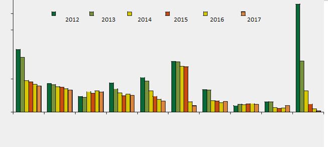 |
|
Source:
Eurostat.
|
|
116
|
MINISTRY
OF ECONOMY AND
FINANCE
|
V. QUALITY
OF PUBLIC
FINANCES
V.1 ACTIONS
TAKEN AND
TRENDS FOR THE
FUTURE YEARS
Measures
adopted in
2018
Various
urgent
measures were
adopted in the
course of
2018. The main
ones provide
for additional
measures in
favour of
people living
in the areas
affected by
the
earthquakes of
2016 and 2017,
actions to
counteract job
insecurity and
protect
employment
levels and
provisions for
fiscal
simplification
and the
extension of
legal
deadlines.
Specific
measures were
also envisaged
to deal with
the state of
emergency
following the
collapse of
the Polcevera
Overpass in
the city of
Genoa, along
with
provisions on
international
protection,
immigration
and public
safety and
actions of
support and
simplification
for businesses
and local
government.
Overall, for
the period
under
consideration,
these measures
lead to slight
improvements
for all public
finance
balances
(Table V.1).
|
TABLE
V.1 -
CUMULATIVE
EFFECTS OF THE
LATEST
MEASURES
IMPLEMENTED IN
2018 ON
GENERAL
GOVERNMENT NET
BORROWING (before
netting out
induced
effects; in €
mn)
|
||||
|
|
2018
|
2019
|
2020
|
2021
|
|
Decree-Law
No. 55/2018
(converted by
Law No.
89/2018)
|
0
|
0
|
0
|
0
|
|
Decree-Law
No. 87/2018
(converted by
Law No.
96/2018)
|
4
|
29
|
0
|
0
|
|
Decree-Law
No. 91/2018
(converted by
Law No.
108/2018)
|
0
|
1
|
0
|
0
|
|
Decree-Law
No. 109/2018
(converted by
Law No.
130/2018)
|
30
|
15
|
12
|
16
|
|
Decree-Law
No. 113/2018
(converted by
Law No.
132/2018)
|
3
|
8
|
9
|
7
|
|
Decree-Law
No. 135/2018
(converted by
Law No.
12/2019)
|
0
|
0
|
1
|
0
|
|
NET
BORROWING
|
38
|
52
|
22
|
23
|
|
% of
GDP
|
0.0
|
0.0
|
0.0
|
0.0
|
|
BORROWING
REQUIREMENT
|
8
|
42
|
22
|
23
|
|
% of
GDP
|
0.0
|
0.0
|
0.0
|
0.0
|
|
NET
BALANCE TO BE
FINANCED
|
40
|
120
|
11
|
19
|
|
% of
GDP
|
0.0
|
0.0
|
0.0
|
0.0
|
|
Note:
Discrepancies,
if any, are
due to
rounding.
|
||||
Incremental
resources
(higher
revenue and
lower
expenditure)
amount to
approximately
0.7 billion in
2018, 1.9
billion in
2019, 1.5
billion in
2020 and 1.4
billion in
2021 (Table
V.2). The
actions taken
(higher
expenditure
and lower
revenue)
amount to
approximately
0.7 billion in
2018, 1.9
billion in
2019, 1.5
billion in
2020 and 1.4
billion in
2021.
|
MINISTRY
OF ECONOMY AND
FINANCE
|
117
|
|
ECONOMIC
AND FINANCIAL
DOCUMENT -
SECT. I STABILITY
PROGRAMME
|
|
TABLE
V.2 -
CUMULATIVE
EFFECTS OF THE
LATEST
MEASURES
IMPLEMENTED IN
2018 ON
GENERAL
GOVERNMENT NET
BORROWING (before
netting out
induced
effects; in €
mn)
|
||||
|
|
2018
|
2019
|
2020
|
2021
|
|
Incremental
resources
|
748
|
1,920
|
1,518
|
1,368
|
|
Higher
revenue
|
181
|
523
|
627
|
674
|
|
Lower
expenditure
|
567
|
1,397
|
890
|
694
|
|
-
current
expenditure
|
274
|
585
|
301
|
258
|
|
-
capital
expenditure
|
292
|
811
|
590
|
436
|
|
Use of
resources
|
710
|
1,868
|
1,496
|
1,346
|
|
Lower
revenue
|
276
|
662
|
659
|
596
|
|
Higher
expenditure
|
434
|
1,207
|
837
|
749
|
|
-
current
expenditure
|
153
|
396
|
238
|
314
|
|
-
capital
expenditure
|
281
|
811
|
599
|
436
|
|
Impact
on net
borrowing
|
38
|
52
|
22
|
23
|
|
Net
change in
revenue
|
-95
|
-138
|
-32
|
78
|
|
Net
change in
expenditure
|
-133
|
-190
|
-53
|
55
|
|
-
current
expenditure
|
-121
|
-189
|
-63
|
55
|
|
-
capital
expenditure
|
-12
|
-1
|
10
|
0
|
|
Note:
Discrepancies,
if any, are
due to
rounding.
|
||||
With
regard to the
subsectors of
general
government
(Table V.3),
the measures
adopted
improve the
net borrowing
of central
government.
The provisions
include, in
particular,
those that
determine an
increase in
the taxes
applicable to
online
gambling
devices and
reductions in
certain State
budget funds.
The deficit of
local
governments
deteriorates
slightly from
2019 to 2021,
primarily due
to the
following
measures:
establishment
of a cash-only
fund to
finance
investments by
local
authorities
through the
use of
administration
results of
previous
years, actions
towards urban
security and
the allocation
of resources
for the
reconstruction
of the
municipalities
affected by
the earthquake
of 21 August
2017. The
negative
impact on the
budget balance
of social
security funds
is due to the
measures in
the field of
labour and
employment.
|
TABLE
V.3 -
CUMULATIVE
EFFECTS OF THE
LATEST
MEASURES
IMPLEMENTED IN
2018 ON
GENERAL
GOVERNMENT NET
BORROWING BY
SUBSECTOR
(before
netting out
induced
effects; in €
mn)
|
||||
|
|
2018
|
2019
|
2020
|
2021
|
|
CENTRAL
GOVERNMENT
|
22
|
153
|
98
|
139
|
|
-net
change in
revenue
|
-46
|
-85
|
53
|
167
|
|
-net
change in
expenditure
|
-68
|
-238
|
-45
|
28
|
|
LOCAL
GOVERNMENT
|
52
|
-19
|
-11
|
-41
|
|
-net
change in
revenue
|
-6
|
-1
|
11
|
15
|
|
-net
change in
expenditure
|
-58
|
18
|
22
|
56
|
|
SOCIAL
SECURITY FUNDS
|
-36
|
-82
|
-65
|
-74
|
|
-net
change in
revenue
|
-43
|
-53
|
-95
|
-103
|
|
-net
change in
expenditure
|
-7
|
29
|
-30
|
-29
|
|
EFFECTS
ON NET
BORROWING
|
38
|
52
|
22
|
23
|
|
Note:
Discrepancies,
if any, are
due to
rounding.
|
||||
Several
measures are
directed
towards
dealing with
emergency
needs. After
the collapse
of a section
of the
Polcevera
Overpass in
the city of
Genoa,
resources
|
118
|
MINISTRY
OF ECONOMY AND
FINANCE
|
|
V. QUALITY
OF PUBLIC
FINANCES
|
were
made available
for an urgent
action plan to
remove and
dispose of the
rubble, design
and rebuild
the road
infrastructure
and restore
the road
system in the
regional
capital of
Liguria1.
Measures
were also
taken to help
the people in
the areas of
Lazio, Marche,
Umbria,
Abruzzo and
Campania
affected by
earthquakes in
2016 and 20172.
These include,
in particular,
extensions and
suspensions of
tax and social
security
payments, and
the
opportunity to
pay the sums
due in
instalments,
in certain
cases. At the
same time,
mortgage
payments due
on loans
granted by
Cassa Depositi
e Prestiti
S.p.a. to the
towns hit by
the
earthquakes
were deferred.
For the
immediate
implementation
of remedial
and security
measures on
motorways A24
and A25, also
affected by
the seismic
events of
recent years,
the resources
originally set
aside for
2022-2025 were
brought
forward to
2018 and 20193.
In the
private sector
of the labour
market, the
total duration
of fixed-term
employment
contracts was
reduced from
36 to 24
months and the
50 percent
exemption on
total social
security
contributions
was extended
(except for
premiums or
contributions
due to INAIL)
for employers
who in 2019
and 2020 hire
workers under
thirty-five
under
permanent
progressive
entitlement
contracts4.
The benefit is
issued for a
maximum of 36
months, up to
a maximum of
3,000 euro
annually. For
fixed-term
employment
contracts,
with the
exception of
domestic work,
there was an
increase of
0.5 percentage
points in
additional
social
security
contribution
to finance the
NASpI, to be
paid by the
employer,
equal to 1.4
per cent of
the
compensation
subject to
social
security
contributions5.
Several
simplification
provisions
were enacted
in the area of
taxation,
including the
deferral to 1
January 2019
of the
electronic
invoicing
obligation for
automotive
fuel purchases
made at
roadside
petrol
stations by
persons liable
for VAT, in
order to
standardize
this sector
with the
general
framework
deadlines set
for other
private
operators. The
provisions on
the exemption
from the VAT
reporting
obligation,
currently
provided only
for residents
of mountainous
areas, were
extended to
all
agricultural
producers. The
split payment
mechanism for
professional
services
provided to
public
administrations
was abolished6.
In order to
counteract VAT
avoidance and
evasion in
business
transactions,
the reverse
tax charge
mechanism was
also extended
to persons
offering the
use of online
platforms,
portals or
similar means
for the sale
of electronic
products to
third parties7.
The entry into
effect of the
provisions
repealing the
reduction in
IRES (CIT,
Corporate
Income Tax)
for some third
sector
organizations
is deferred8.
___
1
Decree-Law No.
109/2018
converted with
amendments by
Law No.
130/2018.
2Decree-Law
No. 55/2018
converted with
amendments by
Law No.
89/2018 and
Decree-Law No.
109/2018
converted with
amendments by
Law No.
130/2018.
3
Decree-Law No.
109/2018
converted with
amendments by
Law No.
130/2018.
4
Decree-Law No.
87/2018
converted with
amendments by
Law No.
96/2018.
5
Other measures
in the labour
market,
provided for
by Decree-Law
No. 87/2018,
also include
the increase
of the maximum
and minimum
compensation
in the event
of unlawful
dismissal.
6
Additional tax
simplification
measures, for
which no
financial
effects on the
General
Government
account are
foreseen,
provide for
procedural
changes
concerning the
institution of
the synthetic
verification
of total
income (redditometro,
or
‘incomemeter’)
and the review
of certain
deadlines for
the
transmission
of data for
invoices
issued and
received
(spesometro,
or
‘spendometer’)
by persons
liable for
VAT.
7
Decree-Law No.
135/2018
converted with
amendments by
Law No.
12/2019.
8
The repeal of
the 50 percent
reduction in
CIT was
initially
provided for
by Article 1,
paragraphs 51
and 52 of the
2019 Budget
Law. Law 12 of
February 2019
under
conversion
into
Decree-Law No.
135/2019 into
law deferred
the run date
of this repeal
until the
entry into
force of
provisions, to
be identified
with
subsequent
measures, in
favour of
non-profit
socially
minded
organizations
and
individuals.
|
MINISTRY
OF ECONOMY AND
FINANCE
|
119
|
|
ECONOMIC
AND FINANCIAL
DOCUMENT -
SECT. I STABILITY
PROGRAMME
|
To
limit gambling
disorders, a
ban was
imposed on any
form of
advertising,
by any means,
of gambling
and betting
with winnings
in cash,
establishing
appropriate
penalties in
the event of
violation9.
Public
safety
measures
include, among
others,
improving the
technical-logistic
devices of the
State Police
and National
Firefighters,
establishing a
fund for the
adoption of
legislative
measures for
the
reorganization
of the roles
and careers of
police and
armed forces
and increasing
the resources
allocated to
municipal
authorities
for the
installation
of video
surveillance
systems10.
For the
continued
support of
Italian
exports in
2018, the fund
managed by
Simest S.p.a
and used for
the
stabilisation
of interest
rates and
exchange rates
in export
credit
transactions
was refinanced11.
Lastly,
the deadline
for repayment
of the
interest
bearing loan
granted to
Alitalia
S.p.a. was
extended to 30
June 201912
and, for 2019,
a contribution
was allocated
to municipal
authorities to
make up for
lost revenue
due to the IMU
first home tax
being replaced
by TASI (tax
on indivisible
municipal
services) on
all property13.
___
9
Decree-Law No.
87/2018
converted with
amendments by
Law No.
96/2018.
10
Decree-Law No.
113/2018
converted with
amendments by
Law No.
132/2018 and
Decree-Law No.
135/2018
converted with
amendments by
Law 12/2019.
11
Decree-Law No.
91/2018
converted with
amendments by
Law No.
108/2018.
12
Decree-Law No.
135/2018
converted with
amendments by
Law No.
12/2019. Since
this concerns
the extension
of the payment
deadline for
the 900
million loan
already
foreseen under
Legislative
Decree No.
50/2017 and
Decree-Law No.
148/2017, the
only financial
effects of the
measure are in
terms of
requirements.
13
Decree-Law No.
135/2018
converted with
amendments by
Law No.
12/2019.
|
120
|
MINISTRY
OF ECONOMY AND
FINANCE
|
|
V. QUALITY
OF PUBLIC
FINANCES
|
|
TABLE
V.4 - EFFECTS
OF DECREE-LAW
NO.109/2018 ON
GENERAL
GOVERNMENT NET
BORROWING
(before
netting out
induced
effects; in €
mn)
|
||||
|
|
2018
|
2019
|
2020
|
2021
|
|
INCREMENTAL
RESOURCES
|
210
|
502
|
199
|
130
|
|
|
|
|
|
|
|
Higher
revenue
|
53
|
11
|
14
|
17
|
|
|
|
|
|
|
|
Sanctions
imposed by the
Italian
Competition
Authority
charged to the
budget
|
49
|
0
|
0
|
0
|
|
National
Agency for the
Safety of
Railways and
Road and
Highway
Infrastructure
- effects of
taxes and
charges
|
0
|
6
|
9
|
9
|
|
Other
|
4
|
5
|
4
|
8
|
|
|
|
|
|
|
|
Lower
expenditure
|
156
|
491
|
185
|
113
|
|
|
|
|
|
|
|
Reduction
of Investment
Fund
|
33
|
185
|
67
|
50
|
|
Change
in Development
and Cohesion
Fund
|
50
|
142
|
0
|
0
|
|
Reduction
of Multiannual
Contribution
Fund
|
52
|
50
|
20
|
0
|
|
Reduction
of Fund for
structural
economic
policy
measures
|
0
|
10
|
50
|
21
|
|
Reduction
of Special
Capital
Account Fund
|
0
|
21
|
20
|
20
|
|
Reduction
of payments to
INAIL for
building
innovative
schools and
children's
centres
|
9
|
14
|
14
|
0
|
|
Reduction
of Special
Current
Account Fund
|
0
|
33
|
1
|
1
|
|
Other
|
12
|
37
|
14
|
21
|
|
|
|
|
|
|
|
USE OF
RESOURCES
|
179
|
487
|
187
|
114
|
|
|
|
|
|
|
|
Lower
revenues
|
17
|
29
|
29
|
0
|
|
|
|
|
|
|
|
Suspension
of deadlines
for payment of
RAI television
fee, social
security and
welfare
contributions,
premiums for
compulsory
insurance and
payment due
notices in
municipalities
hit by the
earthquake of
21 August 2017
|
7
|
28
|
28
|
0
|
|
Urban
Free Trade
Zone in the
metropolitan
city of Genoa
to support
businesses
affected by
the disaster
|
10
|
0
|
0
|
0
|
|
Other
|
0
|
1
|
1
|
0
|
|
|
|
|
|
|
|
Higher
expenditure
|
162
|
458
|
159
|
114
|
|
|
|
|
|
|
|
Expenditure
to reconstruct
the
infrastructure
and restore
the road
system after
the collapse
of part of the
Polcevera
Overpass
|
40
|
180
|
80
|
0
|
|
Restoration
and
implementation
of safety
measures for
motorways A24
and A25 after
the
earthquakes of
2009, 2016 and
2017
|
50
|
142
|
0
|
0
|
|
Provisions
on local
public
transport,
road haulage
and road
conditions for
the city of
Genoa
|
26
|
43
|
0
|
0
|
|
Increase
of Fund for
reconstruction
operations in
the
municipalities
of
Casamicciola
Terme, Forio
and Lacco
Ameno hit by
the earthquake
of 21 August
2017
|
0
|
20
|
20
|
20
|
|
National
Agency for the
Safety of
Railways and
Road and
Highway
Infrastructure
|
0
|
14
|
22
|
22
|
|
Increase
of Multiannual
Contribution
Fund
|
0
|
0
|
0
|
50
|
|
Design
of innovative
schools and
children's
centres
|
9
|
14
|
14
|
0
|
|
Optimization
of logistic
traffic flows
in the port of
Genoa
|
8
|
15
|
7
|
0
|
|
Other
|
30
|
30
|
16
|
21
|
|
|
|
|
|
|
|
IMPACT
ON NET
BORROWING
|
30
|
15
|
12
|
16
|
|
Note:
Discrepancies,
if any, are
due to
rounding.
|
|
|
|
|
|
MINISTRY
OF ECONOMY AND
FINANCE
|
121
|
|
ECONOMIC
AND FINANCIAL
DOCUMENT -
SECT. I STABILITY
PROGRAMME
|
|
TABLE
V.5 - EFFECTS
OF DECREE-LAW
NO.113/2018 ON
GENERAL
GOVERNMENT NET
BORROWING
(before
netting out
induced
effects; in €
mn)
|
||||
|
|
2018
|
2019
|
2020
|
2021
|
|
INCREMENTAL
RESOURCES
|
101
|
128
|
145
|
147
|
|
|
|
|
|
|
|
Higher
revenue
|
25
|
15
|
16
|
14
|
|
|
|
|
|
|
|
Fund
for the
reorganisation
of the roles
and careers of
police and
armed forces -
effects of
taxes and
charges
|
24
|
10
|
10
|
10
|
|
Other
|
1
|
6
|
7
|
4
|
|
|
|
|
|
|
|
Lower
expenditure
|
76
|
112
|
128
|
133
|
|
|
|
|
|
|
|
Reduction
of Special
Capital
Account Fund
|
17
|
64
|
74
|
74
|
|
Reduction
of Public
Employee
Contract Fund
|
45
|
15
|
15
|
15
|
|
Reduction
of Special
Current
Account Fund
|
5
|
6
|
5
|
5
|
|
Other
|
9
|
27
|
34
|
39
|
|
|
|
|
|
|
|
USE OF
RESOURCES
|
98
|
120
|
136
|
141
|
|
|
|
|
|
|
|
Lower
revenue
|
22
|
7
|
7
|
7
|
|
|
|
|
|
|
|
Fund
for public
employee
contracts -
effects of
taxes and
charges
|
22
|
7
|
7
|
7
|
|
|
|
|
|
|
|
Higher
expenditure
|
76
|
112
|
128
|
133
|
|
|
|
|
|
|
|
Purchase
and
improvement of
information
systems for
combating
international
terrorism and
financing the
extraordinary
maintenance
and adaptation
of structures
and
installations
- State Police
and Fire
Brigade
|
15
|
49
|
49
|
49
|
|
Fund
for the
reorganization
of the roles
and careers of
police and
armed forces
|
50
|
20
|
20
|
20
|
|
Measures
for improving
and
implementing
safety
measures for
prison
facilities
|
7
|
15
|
25
|
25
|
|
Urban
safety
operations:
installation
of video
surveillance
systems by
Municipal
Authorities
|
0
|
10
|
17
|
27
|
|
Other
|
4
|
18
|
17
|
12
|
|
|
|
|
|
|
|
IMPACT
ON NET
BORROWING
|
3
|
8
|
9
|
7
|
|
Note:
Discrepancies,
if any, are
due to
rounding.
|
||||
|
122
|
MINISTRY
OF ECONOMY AND
FINANCE
|
|
V. QUALITY
OF PUBLIC
FINANCES
|
|
TABLE
V.6 - EFFECTS
OF DECREE-LAW
NO.135/2018 ON
GENERAL
GOVERNMENT NET
BORROWING (before
netting out
induced
effects; in €
mn)
|
||||
|
|
2018
|
2019
|
2020
|
2021
|
|
INCREMENTAL
RESOURCES
|
12
|
351
|
273
|
274
|
|
|
|
|
|
|
|
Higher
revenue
|
4
|
77
|
103
|
102
|
|
|
|
|
|
|
|
Counteracting
VAT avoidance
and evasion in
business
transactions
performed
through online
trading
platforms
|
0
|
72
|
86
|
86
|
|
Other
|
4
|
5
|
17
|
16
|
|
|
|
|
|
|
|
Lower
expenditure
|
8
|
274
|
169
|
171
|
|
|
|
|
|
|
|
Reduction
of Fund for
structural
economic
policy
measures
|
0
|
108
|
131
|
78
|
|
Reduction
of Fund to
meet
non-deferrable
expenditure
|
0
|
0
|
12
|
86
|
|
Reduction
of Citizen's
Income Fund
|
0
|
90
|
0
|
0
|
|
Reduction
of Government
Programme
Implementation
Fund
|
0
|
20
|
17
|
0
|
|
Other
|
8
|
55
|
10
|
8
|
|
|
|
|
|
|
|
USE OF
RESOURCES
|
12
|
351
|
272
|
274
|
|
|
|
|
|
|
|
Lower
revenue
|
4
|
123
|
158
|
159
|
|
|
|
|
|
|
|
Deferral
of effective
date of
reduction in
CIT subsidies
for
non-commercial
bodies
|
0
|
118
|
158
|
158
|
|
Other
|
4
|
4
|
0
|
1
|
|
|
|
|
|
|
|
Higher
expenditure
|
8
|
228
|
114
|
115
|
|
|
|
|
|
|
|
Increase
of Government
Programme
Implementation
Fund
|
0
|
72
|
86
|
86
|
|
Contribution
to Municipal
Authorities to
make up for
lower revenue
due to the
introduction
of the TASI
|
0
|
110
|
0
|
0
|
|
Plan
for the
transition to
sustainable
energy
|
0
|
1
|
16
|
15
|
|
Increase
in funds for
urban safety
|
0
|
20
|
0
|
0
|
|
Other
|
8
|
25
|
12
|
14
|
|
|
|
|
|
|
|
IMPACT
ON NET
BORROWING
|
0
|
0
|
1
|
0
|
|
Note:
Discrepancies,
if any, are
due to
rounding.
|
||||
The
2019-2021
public finance
Budget and
initial
measures in
2019: impact
on balances
The
public finance
Budget for
2019-2021 is
composed of
the provisions
of the 2019
Budget Law14,
as well as the
financial
effects of
Decree-Law No.
119/201815
laying down
urgent tax and
financial
provisions.
Overall,
the public
finance Budget
and the first
measures
undertaken in
201916
(Table V.7)
lead to an
increase in
net borrowing
of
approximately
11.5
___
14
Law No.
145/2018.
15
Converted with
amendments by
Law No.
136/2018.
16
In the course
of 2019, other
measures were
also adopted
with
substantially
neutral
effects on
public finance
balances.
These include
Decree-
|
MINISTRY
OF ECONOMY AND
FINANCE
|
123
|
|
ECONOMIC
AND FINANCIAL
DOCUMENT -
SECT. I STABILITY
PROGRAMME
|
billion
in 2019, 14.4
billion in
2020 and 9.2
billion in
2021. The
expected
deterioration
in the
borrowing
requirement is
approximately
12.8 billion
in 2019, 15.6
billion in
2020 and 9.5
billion in
2021. The
State budget
shows an
increase in
the net
balance to be
financed of
approximately
19.5 billion
in 2019 and
14.3 billion
in 2020 and in
202117.
|
TABLE
V.7 - EFFECTS
OF THE
2019-2021
PUBLIC FINANCE
BUDGET AND
INITIAL
MEASURES IN
2019 (before
netting out
induced
effects; in €
mn)
|
||||
|
|
2018
|
2019
|
2020
|
2021
|
|
2019
Budget Law
(Law
No.145/2018)
|
0
|
-11,586
|
-14,551
|
-9,290
|
|
Decree-Law
No.119/2018
(cvt. by Law
No.136/2018)
|
7
|
42
|
43
|
55
|
|
Decree-Law
No. 4/2019 (cvt.
by Law No.
26/2019)
|
0
|
7
|
77
|
54
|
|
|
|
|
|
|
|
NET
BORROWING
|
7
|
-11,537
|
-14,431
|
-9,180
|
|
% of
GDP
|
0.0
|
-0.6
|
-0.8
|
-0.5
|
|
BORROWING
REQUIREMENT
|
442
|
-12,822
|
-15,554
|
-9,542
|
|
% of
GDP
|
0.0
|
-0.7
|
-0.9
|
-0.5
|
|
NET
BALANCE TO BE
FINANCED
|
177
|
-19,450
|
-14,315
|
-14,283
|
|
% of
GDP
|
0.0
|
-1.1
|
-0.8
|
-0.8
|
|
Note:
Discrepancies,
if any, are
due to
rounding.
|
||||
In
terms of
accounting,
funding for
the public
finance Budget
(higher
revenue and
lower
expenditure)
amounted to
approximately
29.7 billion
in 2019, 34.9
billion in
2020 and 40.3
billion in
2021 (Table
V.8). The
actions
financed
(lower revenue
and higher
expenditure),
equal to
approximately
41.2 billion
in 2019, 49.4
billion in
2020 and 49.5
billion in
2021, are
aimed at
supporting
economic
growth by
reducing the
tax burden and
reviving
private and
public
investment and
at providing
new social
security and
social
inclusion
measures, the
implementation
of which is
defined by
Decree-Law No.
4/2019 (Table
V.8a) through
the use of
resources
allocated in
special State
budget funds.
Law No.
1/2019
converted with
amendments by
Law No.16/2019
laying down
urgent
measures to
support Banca
Carige S.p.a.
- Cassa di
Risparmio di
Genova e
Imperia,
Decree-Law No.
22/2019 laying
down urgent
measures to
ensure the
safety,
financial
stability and
integrity of
markets as
well as the
protection of
the health and
freedom of
residence of
Italian and
British
citizens in
the event of
withdrawal of
the UK from
the European
Union and
Decree-Law No.
27/2019 laying
down urgent
provisions to
revive the
agricultural
sectors in
crisis and
support farms
affected by
particularly
extreme
weather events
and for the
emergency
situation at
the Stoppani
factory in
Cogoleto.
17
The different
impact on
State budget
requirement
and net
balance to be
financed with
regard to net
borrowing is
due to the
different
accounting
criteria for
transactions
carried out on
these
aggregates and
to the fact
that they
refer to
different
institutional
aggregates.
|
124
|
MINISTRY
OF ECONOMY AND
FINANCE
|
|
V. QUALITY
OF PUBLIC
FINANCES
|
|
TABLE
V.8 - EFFECTS
OF THE
2019-2021
PUBLIC FINANCE
BUDGET ON
GENERAL
GOVERNMENT NET
BORROWING
(before
netting out
induced
effects; in €
mn)
|
||||
|
|
2018
|
2019
|
2020
|
2021
|
|
INCREMENTAL
RESOURCES
|
1,797
|
29,691
|
34,862
|
40,276
|
|
Higher
revenue
|
223
|
14,286
|
21,014
|
25,654
|
|
Lower
expenditure
|
1,574
|
15,405
|
13,848
|
14,622
|
|
current
expenditure
|
1,047
|
7,864
|
9,672
|
10,495
|
|
capital
expenditure
|
527
|
7,541
|
4,176
|
4,126
|
|
USE OF
RESOURCES
|
1,790
|
41,235
|
49,370
|
49,511
|
|
Lower
revenue
|
565
|
18,229
|
12,804
|
13,871
|
|
Higher
expenditure
|
1,225
|
23,006
|
36,566
|
35,640
|
|
current
expenditure
|
170
|
17,524
|
26,128
|
24,392
|
|
capital
expenditure
|
1,055
|
5,482
|
10,439
|
11,248
|
|
IMPACT
ON NET
BORROWING
|
7
|
-11,544
|
-14,508
|
-9,235
|
|
Change
net in revenue
|
-342
|
-3,943
|
8,210
|
11,784
|
|
Change
net in
expenditure
|
-349
|
7,601
|
22,719
|
21,018
|
|
current
expenditure
|
-877
|
9,660
|
16,456
|
13,897
|
|
capital
expenditure
|
528
|
-2,059
|
6,263
|
7,122
|
|
Note:
Discrepancies,
if any, are
due to
rounding.
The
2019-2021
public finance
Budget
includes the
effects of the
2019 Budget
Law and
Decree-Law No.
119/2018
converted by
Law No.
136/2018.
|
||||
|
TABLE
V.8A - EFFECTS
OF DECREE-LAW
NO. 4/2019 ON
GENERAL
GOVERNMENT NET
BORROWING
(before
netting out
induced
effects;
values in € m)
|
||||
|
|
2018
|
2019
|
2020
|
2021
|
|
INCREMENTAL
RESOURCES
|
0
|
11,204
|
16,594
|
17,309
|
|
Higher
revenue
|
0
|
748
|
672
|
678
|
|
Lower
expenditure
|
0
|
10,456
|
15,922
|
16,631
|
|
current
expenditure
|
0
|
10,447
|
15,922
|
16,631
|
|
capital
expenditure
|
0
|
9
|
0
|
0
|
|
USE OF
RESOURCES
|
0
|
11,198
|
16,517
|
17,254
|
|
Lower
revenue
|
0
|
14
|
170
|
278
|
|
Higher
expenditure
|
0
|
11,183
|
16,347
|
16,976
|
|
current
expenditure
|
0
|
11,183
|
16,347
|
16,976
|
|
capital
expenditure
|
0
|
0
|
0
|
0
|
|
IMPACT
ON NET
BORROWING
|
0
|
7
|
77
|
54
|
|
Change
net in revenue
|
0
|
734
|
502
|
400
|
|
Change
net in
expenditure
|
0
|
727
|
425
|
346
|
|
current
expenditure
|
0
|
737
|
425
|
346
|
|
capital
expenditure
|
0
|
-9
|
0
|
0
|
|
Note:
Discrepancies,
if any, are
due to
rounding.
|
||||
With
regard to
general
government
subsectors,
the Budget Law
and Decree-Law
No. 4/2019 are
substantially
neutral on the
budget balance
of central
government in
2019 and
entail an
improvement of
around 3.6
billion in
2020 and 8.5
billion in
2021. This
result depends
predominantly
on the
deactivation
of the
safeguard
clauses for
the 2019 and
their
recalculation
with effect
from 2020.
Moreover, the
review of
certain
transfers and
funds of the
State budget
and the
resources for
financing
investment by
the central
administrations
of the State
and for
contract
renewals and
recruitment of
personnel in
the public
sector all
have an impact
on spending.
|
MINISTRY
OF ECONOMY AND
FINANCE
|
125
|
|
ECONOMIC
AND FINANCIAL
DOCUMENT -
SECT. I STABILITY
PROGRAMME
|
These
measures
involve a
deficit
increase for
local
government of
around 1.2
billion in
2019, 4.3
billion in
2020 and 4.0
billion in
2021, due
essentially to
the provisions
to stimulate
the revival of
investment by
regional and
local
authorities.
The
negative
impact on the
deficit of
Social
security funds
is
approximately
10.3 billion
in 2019, 13.8
billion in
2020 and 13.7
billion in
2021, as a
result of the
new early
retirement
provision and
the
institution of
Citizen's
Income.
|
TABLE
V.9 - EFFECTS
OF THE
2019-2021
PUBLIC
FINANCE
BUDGET AND
INITIAL
MEASURES IN
2019 ON
GENERAL
GOVERNMENT NET
BORROWING BY
SUBSECTOR
(before
netting out
induced
effects; in €
mn)
|
||||
|
2018
|
2019
|
2020
|
2021
|
|
|
CENTRAL
GOVERNMENT
|
-209
|
-32
|
3,599
|
8,519
|
|
change
in net revenue
|
-241
|
-4,097
|
7,637
|
11,593
|
|
change
in net
expenditure
|
-32
|
-4,065
|
4,037
|
3,074
|
|
|
|
|
|
|
|
LOCAL
GOVERNMENT
|
298
|
-1,188
|
-4,258
|
-3,983
|
|
change
in net revenue
|
-1
|
1,084
|
456
|
77
|
|
change
in net
expenditure
|
-298
|
2,271
|
4,714
|
4,059
|
|
Table
|
|
|
|
|
|
SOCIAL
SECURITY FUNDS
|
-81
|
-10,317
|
-13,773
|
-13,717
|
|
change
in net revenue
|
-100
|
-195
|
619
|
514
|
|
change
in net
expenditure
|
-19
|
10,122
|
14,392
|
14,231
|
|
|
|
|
|
|
|
EFFECTS
ON NET
BORROWING
|
7
|
-11,537
|
-14,431
|
-9,180
|
|
Note:
Discrepancies,
if any, are
due to
rounding.
|
||||
The
2019-2021
public finance
Budget: main
measures
The
2019-2021
public finance
Budget (Table
V.10) provides
for a series
of actions to
reduce the tax
burden on
citizens and
businesses.
These
include the
complete
deactivation
of the
so-called
safeguard
clauses
(automatic
increases in
VAT rates and
excise duties
on fuel) for
2019 for a
total of 12.5
billion. At
the same time,
the scope of
the subsidised
flat-rate tax
scheme is
extended,
raising the
eligibility
threshold of
revenue and
remunerations
to 65,000 euro
(in net terms,
0.3 billion in
2019, 1.8
billion in
2020 and 1.4
billion in
2021), while a
single 20
percent income
tax rate is
introduced,
replacing
current taxes
for individual
business
entrepreneurs,
artists and
professionals
earning 65,000
to 100,000
euro
(approximately
0.1 billion in
2020 and 1.13
billion in
2021). To help
businesses, a
subsidised 15
percent tax
rate is
applied to
income
reinvested to
purchase
exclusively
tangible
capital goods
(excluding
non-company
property and
vehicles) and
to increase
fixed-term and
permanent
employment
(approximately
1.9 billion in
2020 and 1.8
billion in
2021). In
addition, the
proportion of
IMU property
tax paid on
company
property
deductible for
CIT and PIT
(Personal
Income Tax)
purposes is
increased from
20 to 40
percent (0.3
billion in
2020 and 0.2
billion in
2021).
To
promote
competitiveness
and
development,
tax deductions
are extended
to 2019 for
expenses due
to energy
efficiency
operations,
building
renovations,
|
126
|
MINISTRY
OF ECONOMY AND
FINANCE
|
|
V. QUALITY
OF PUBLIC
FINANCES
|
the
purchase of
furniture and
re-greening
(approximately
0.6 billion in
2020 and 0.9
billion in
2021), as well
as subsidies
for
investments in
new tangible
capital assets
and intangible
asset for the
technological
transformation
of businesses
(also known as
‘hyper-amortisation’),
envisaging the
simultaneous
restructuring
of the tax
benefit
granted, and
subsidies for
the purchase
of intangible
capital goods
that are
classified
within the
category of
specific
software (also
known as
‘super-amortisation’)
with an
overall impact
of
approximately
0.4 billion in
2020 and 0.8
billion in
2021. A
reduction in
the rate of
premiums
against
accidents at
work and
occupational
diseases
managed by
INAIL is also
envisaged for
the 3-year
period
2019-2021 only
(in net terms,
approximately
0.4 billion in
2019 and 2020
and 0.5
billion in
2021).
As for
welfare and
assistance,
special funds
are foreseen
for the
introduction
of the
Citizen's
Income and
Citizen's
Pension
(approximately
7.1 billion in
2019, 8.1
billion in
2020 and 8.2
billion in
2021) and for
the definition
of additional
types of early
retirement
(approximately
4 billion in
2019, 8.3
billion in
2020 and 8.7
billion in
2021).
Decree-Law No.
4/2019 has
identified the
implementing
measures for
disbursing the
expenditure
(see the next
paragraph for
more details).
Furthermore,
in terms of
social
measures, the
following
funds are
refinanced:
the fund for
dependants and
caregivers
(0.1 billion
annually from
2019); the
fund for
social
policies (0.1
billion
annually from
2019); the
fund for
family
policies (0.1
billion
annually from
2019); and the
fund for
supporting
students with
physical and
sensory
disabilities
(0.1 billion
annually for
the period
2019-2021). In
addition, the
maternity
allowance,
also known as
the ‘Baby
bonus’, is
also extended
to 2019
(approximately
0.2 billion in
2019 and
2020).
As for
public
employment,
resources have
been set aside
for: the
national
collective
bargaining for
2019-2021 and
economic
improvements
for central
government
employees
(approximately
0.7 billion in
2019, 0.9
billion in
2020 and 1.3
billion in
2021, which,
net of taxes
and social
security
contributions,
correspond to
0.3 billion in
2019, 0.5
billion in
2020 and 0.7
billion
starting from
2021); and for
the
recruitment of
State sector
personnel
(also
considering
the costs of
insolvency
proceedings,
approximately
0.3 billion in
2019, 0.9
billion in
2020 and 1.1
billion in
2021, which,
net of taxes
and social
security
contributions,
correspond to
0.1 billion in
2019, 0.5
billion in
2020 and 0.6
billion in
2021).
To
sustain the
investments of
central
administrations
of the Stare,
a special fund
is
established,
to be divided
with one or
more decrees
by the Prime
Minister, with
an impact on
net borrowing
of
approximately
0.4 billion in
2019, 1.2
billion in
2020 and 1.7
billion in
2021 (against
State budget
allocations of
approximately
43.6 billion
in the period
2019-2033).
Furthermore,
expenditure is
foreseen to
mitigate
hydraulic and
hydrogeological
risks (0.6
billion in
2019, 0.8
billion in
2020 and 0.9
billion in
2021) and to
implement the
initial step
of the
National Plan
of Operations
in the Water
Sector
provided by
the 2018
Budget Law
(0.1 billion
per year from
2019 to 2028).
The
following are
envisaged to
boost
investment by
local
governments:
‘release’ of
the
administration
surpluses of
regional and
local
authorities
(0.4 billion
in 2020 and
0.7 billion in
2021);
reduction of
the
ordinary-statute
regions’
contributions
to public
finance for
2019 and 2020,
ordering the
simultaneous
assignment of
a contribution
and the
obligation to
achieve a
positive
budget
|
MINISTRY
OF ECONOMY AND
FINANCE
|
127
|
|
ECONOMIC
AND FINANCIAL
DOCUMENT -
SECT. I STABILITY
PROGRAMME
|
balance
(altogether,
around 0.8
billion in
2019, 1.7
billion in
2020 and 1
billion in
2021) and
other measures
for a total of
0.9 billion in
2019, 0,7
billion in
2020 and 1.2
billion in
2021,
including the
maintenance
and security
of roads,
schools and
the measures
for rewarding
regional
investment.
Resources
are also
provided for
emergencies,
in particular
in relation to
the recent
earthquakes
and floods,
support for
the people of
Genova for the
damage caused
by the
collapse of
the Polcevera
Overpass and
seismic risk
prevention
measures (a
total of about
1 billion in
2019 and 0.6
billion in
2020 and
2021).
Finally,
other actions
include the
1.5 billion
refinancing of
international
missions for
2020 (1.1
billion net of
taxes and
social
security
contributions)
and new
measures to
refund
investors who
have suffered
unjust damage
as a result of
purchasing
financial
instruments
issued by
banks
subjected to
resolution (in
net terms,
around 0.05
billion in
2019, 0.3
billion in
2020 and 0.4
billion in
2021 compared
to the
corresponding
budgetary
allocation of
about 0.5
billion per
year in the
three-year
period)
|
128
|
MINISTRY
OF ECONOMY AND
FINANCE
|
|
V. QUALITY
OF PUBLIC
FINANCES
|
|
TABLE
V.10 -
EFFECTS OF THE
2019-2021
PUBLIC FINANCE
BUDGET ON
GENERAL
GOVERNMENT NET
BORROWING
(before
netting out
induced
effects; in €
mn)
|
||||
|
|
2018
|
2019
|
2020
|
2021
|
|
INCREMENTAL
RESOURCES
|
1,797
|
29,691
|
34,862
|
40,276
|
|
Higher
revenue
|
223
|
14,286
|
21,014
|
25,654
|
|
Revision
of VAT clauses
and excise
duties for
fuel
|
0
|
0
|
3,910
|
9,182
|
|
Repeal
of optional
corporate
income tax
(IRI) regime
|
0
|
5,332
|
3,112
|
3,116
|
|
Repeal
of ACE
|
0
|
228
|
2,373
|
1,453
|
|
Extension
of facilitated
tax regime to
individuals
with revenue
up to 65,000
euro
|
0
|
232
|
2,150
|
1,229
|
|
Obligation
to store and
transmit fees
electronically
|
0
|
337
|
1,356
|
1,912
|
|
Restructuring
of deduction
of start-up
amortisation
and other
intangible
assets
|
0
|
1,308
|
926
|
658
|
|
Subsidised
definition of
collection
agent charges
|
0
|
37
|
1,083
|
1,385
|
|
Substitute
tax for
individual
entrepreneurs
and artists
and
professionals
|
0
|
0
|
280
|
1,918
|
|
Provisions
on gambling
|
0
|
768
|
695
|
695
|
|
Formalisation
of
infringements,
non-conformities,
irregularities
or fulfilments
of a formal
nature
|
0
|
810
|
540
|
0
|
|
Web tax
|
0
|
150
|
600
|
600
|
|
Regulation
of the
deductibility
of credit
write-downs in
the first
application of
IFRS 9
|
0
|
1,170
|
0
|
0
|
|
Revaluation
of insurance
tax account
|
0
|
832
|
0
|
320
|
|
Deferment
to 2026 of 10%
deductibility
of credit
write-downs
|
0
|
950
|
0
|
0
|
|
Extension
of deductions
for building
renovation
energy
efficiency
improvements,
re-greening
and purchase
of furniture
and household
electrical
goods
|
0
|
157
|
697
|
0
|
|
Revaluation
of value of
non-traded
equity
interests and
land
|
0
|
341
|
185
|
185
|
|
Broadband
- greater
revenue from
5G frequencies
|
0
|
200
|
200
|
200
|
|
Flat-rate
tax on income
from letting
commercial
property
|
0
|
0
|
396
|
203
|
|
Reduction
in CIT
subsidies for
non-commercial
entities
|
0
|
118
|
158
|
158
|
|
Increase
in tobacco
excise duties
|
0
|
135
|
135
|
135
|
|
Revision
of the tariffs
of INAIL
premiums and
contributions
for insurance
against
accidents at
work and
occupational
diseases - tax
effects
|
0
|
0
|
174
|
147
|
|
Pending
litigation
|
0
|
78
|
104
|
104
|
|
Increase
in rates of
replacement
tax on the
revaluation of
land and
equity
interest
|
0
|
116
|
63
|
63
|
|
Tax on
the purchase
of highly
polluting
vehicles
|
0
|
62
|
74
|
74
|
|
Tax on
money
transfers
abroad
|
63
|
63
|
63
|
|
|
Subsidised
definition of
formal reports
and notices
|
0
|
51
|
68
|
68
|
|
Change
of accounts of
flat-rate tax
on rents
|
0
|
0
|
0
|
116
|
|
Balance
and write-off
of collection
agent charges
from 2000 to
2017 for
persons with
ISEE <
20,000 euro
|
0
|
43
|
43
|
17
|
|
Job
centre
recruitment -
effects of
taxes and
charges
|
0
|
150
|
150
|
228
|
|
Recruitment
in national
government -
effects of
taxes and
charges
|
0
|
127
|
449
|
547
|
|
Study
grants for
specialist
trainee
doctors -
effects of
taxes and
charges
|
0
|
11
|
22
|
33
|
|
Emergency
requirements -
effects of
taxes and
charges
|
0
|
30
|
40
|
0
|
|
Fund for
international
missions -
effects of
taxes and
charges
|
41
|
0
|
350
|
0
|
|
Fund for
ordinary
financing of
universities -
effects of
taxes and
charges
|
0
|
10
|
28
|
28
|
|
Renewal
of public
employee
contracts for
2019-2021 -
effects of
taxes and
charges
|
0
|
315
|
449
|
618
|
|
Reorganization
of the roles
and careers of
police and
armed forces -
effects of
taxes and
charges
|
0
|
0
|
49
|
49
|
|
Other
|
182
|
128
|
93
|
151
|
|
Note:
Discrepancies,
if any, are
due to
rounding. The
2019-2021
public finance
Budget
includes the
effects of the
2019 Budget
Law and
Decree-Law No.
119/2018
converted by
Law No.
136/2018.
|
||||
|
MINISTRY
OF ECONOMY AND
FINANCE
|
129
|
|
ECONOMIC
AND FINANCIAL
DOCUMENT -
SECT. I STABILITY
PROGRAMME
|
|
TABLE
V.10
(CONTINUED 1)-
EFFECTS OF THE
2019-2021
PUBLIC FINANCE
BUDGET ON
GENERAL
GOVERNMENT NET
BORROWING
(before
netting out
induced
effects; in €
mn)
|
||||
|
2018
|
2019
|
2020
|
2021
|
|
|
|
|
|
|
|
|
Lower
expenditure
|
1,574
|
15,405
|
13,848
|
14,622
|
|
|
|
|
|
|
|
Poverty
Fund (share
merged into
the Citizen's
Income Fund)
|
0
|
2,198
|
2,158
|
2,130
|
|
Local
Authority
Investment
Fund
(reduction for
measures in
favour of
Local
Authorities)
|
0
|
1,080
|
2,342
|
2,249
|
|
Fund
for reducing
the tax burden
|
0
|
390
|
1,639
|
2,472
|
|
Reduction
of
ordinary-statute
regional
authority
contributions
to public
finances
(non-transfer
of the
contribution
to boost
public
investment and
achievement of
a positive
budget
balance)
|
0
|
2,496
|
1,746
|
0
|
|
Pension
indexation
cooling
|
0
|
415
|
1,222
|
2,014
|
|
Ministry
spending
rationalization
measures
|
819
|
915
|
930
|
892
|
|
Reprogramming
of State
transfers
|
0
|
2,340
|
0
|
0
|
|
Reduction
of fund for
implementing
multiannual
contributions
|
0
|
33
|
802
|
992
|
|
Development
and Cohesion
Fund
|
300
|
1,335
|
0
|
0
|
|
Rationalization
of expenditure
for the
management of
immigration
centres
|
0
|
400
|
550
|
650
|
|
Decommissioning
of public
property
|
0
|
950
|
150
|
150
|
|
Determination
of trend at
unchanged
legislation of
National
Health Service
financing
2019-2021
|
0
|
0
|
175
|
1,000
|
|
Complementary
programmes for
action and
cohesion plans
|
0
|
850
|
0
|
0
|
|
Amendment
to research
and
development
tax credit
regulations
|
0
|
0
|
300
|
300
|
|
Fund
for the
purchase of
cleaning
services in
schools
|
0
|
0
|
280
|
280
|
|
Repeal
of tax credit
for IRAP
(regional tax
on productive
activities)
taxpayers
without
employees
|
0
|
163
|
163
|
163
|
|
Reduction
of annual
pensions
exceeding
100,000 euro
gross
|
0
|
138
|
145
|
152
|
|
Reduction
of structural
resources
provided by
INAIL for the
financing of
investment and
training
projects on
occupational
safety and
health
|
0
|
110
|
100
|
100
|
|
Reduction
and
reprogramming
of military
expenditure
|
0
|
103
|
120
|
76
|
|
Deferment
of public
sector
recruitment
|
0
|
198
|
0
|
0
|
|
Citizen's
Income Fund
|
0
|
0
|
0
|
160
|
|
Reduction
of Fund to
meet
non-deferrable
expenditure
|
5
|
0
|
0
|
130
|
|
Investor
Compensation
Fund
|
0
|
26
|
26
|
26
|
|
Other
|
451
|
1,264
|
999
|
686
|
|
Note:
Discrepancies,
if any, are
due to
rounding. The
2019-2021
public finance
Budget
includes the
effects of the
2019 Budget
Law and
Decree-Law No.
119/2018
converted by
Law No
136/2018.
|
||||
|
130
|
MINISTRY
OF ECONOMY AND
FINANCE
|
|
V. QUALITY
OF PUBLIC
FINANCES
|
|
TABLE
V.10
(CONTINUED 2)
- EFFECTS OF
THE 2019-2021
PUBLIC FINANCE
BUDGET ON
GENERAL
GOVERNMENT NET
BORROWING
(before
netting out
induced
effects; in €
mn)
|
||||
|
|
2018
|
2019
|
2020
|
2021
|
|
|
|
|
|
|
|
USE OF
RESOURCES
|
1,790
|
41,235
|
49,370
|
49,511
|
|
|
|
|
|
|
|
Lower
revenue
|
565
|
18,229
|
12,804
|
13,871
|
|
|
|
|
|
|
|
Sterilization
of VAT clauses
and excise
duties for
fuel
|
0
|
12,472
|
0
|
0
|
|
Extension
of facilitated
tax regime to
individuals
with revenue
up to 65,000
euro
|
0
|
563
|
3,971
|
2,603
|
|
Repeal
of optional
regime of
corporate
income tax
(IRI)
|
0
|
3,345
|
1,876
|
1,857
|
|
Subsidised
15% taxation
on the
proportion of
income
corresponding
to profits
invested in
capital assets
|
0
|
0
|
1,948
|
1,808
|
|
Substitute
tax for
individual
entrepreneurs
and artists
and
professionals
|
0
|
0
|
389
|
3,050
|
|
Extension
of deductions
for building
renovation,
energy
efficiency
improvements,
re-greening
and purchase
of furniture
and household
electrical
goods
|
0
|
121
|
1,292
|
887
|
|
Revision
of the rates
for INAIL
premiums and
contributions
for insurance
against
accidents at
work and
occupational
diseases
|
0
|
410
|
525
|
600
|
|
Pension
indexation
cooling - tax
effects
|
0
|
162
|
477
|
786
|
|
Extension
of
hyper-amortisation
and
super-amortisation
|
0
|
0
|
405
|
810
|
|
Flat-rate
tax on income
from letting
commercial
property
|
0
|
261
|
369
|
367
|
|
Up to
40%
deductibility
of IMU for
company
property for
RES and PIT
purposes
|
0
|
0
|
290
|
167
|
|
Repeal
of increase in
excise duties
for fuels
|
0
|
141
|
146
|
148
|
|
Subsidised
definition of
collection
agent charges
|
355
|
20
|
13
|
11
|
|
Formalisation
of
infringements,
non-conformities,
irregularities
or fulfilments
of a formal
nature
|
0
|
130
|
130
|
130
|
|
Revaluation
of insurance
tax account
|
0
|
0
|
320
|
0
|
|
Regulation
of
deductibility
of credit
write-downs in
the first
application of
IFRS 9
|
0
|
0
|
130
|
130
|
|
Review
of the
regulation of
reportable tax
losses
|
0
|
143
|
12
|
102
|
|
Emergency
requirements
|
0
|
119
|
86
|
35
|
|
Tax
on the
consumption of
tobacco
substitutes
|
0
|
70
|
70
|
70
|
|
Reduction
of annual
pensions
exceeding
100,000 euro
gross - tax
effects
|
0
|
62
|
65
|
68
|
|
Other
investment
support
measures
|
0
|
10
|
48
|
38
|
|
Balance
and write-off
of collection
agent charges
from 2000 to
2017 for
persons with
ISEE <
20,000 euro
|
0
|
5
|
5
|
25
|
|
Deferment
of public
sector
recruitment -
effects of
taxes and
charges
|
0
|
97
|
0
|
0
|
|
Ministry
expenditure
rationalization
- effects of
taxes and
charges
|
6
|
11
|
34
|
34
|
|
Other
|
204
|
87
|
201
|
146
|
|
Note:
Discrepancies,
if any, are
due to
rounding.
The
2019-2021
public finance
Budget
includes the
effects of the
2019 Budget
Law and
Decree-Law No.
119/2018
converted by
Law No.
136/2018.
|
||||
|
MINISTRY
OF ECONOMY AND
FINANCE
|
131
|
|
ECONOMIC
AND FINANCIAL
DOCUMENT -
SECT. I STABILITY
PROGRAMME
|
|
Table
V.10
(CONTINUED 3):
EFFECTS OF THE
2019-2021
PUBLIC FINANCE
BUDGET ON
GENERAL
GOVERNMENT NET
BORROWING
before netting
out induced
effects; in €
mn)
|
||||
|
|
2018
|
2019
|
2020
|
2021
|
|
Higher
expenditure
|
1,225
|
23,006
|
36,566
|
35,640
|
|
Citizen's
Income Fund*
|
0
|
7,100
|
8,055
|
8,317
|
|
Pension
System Review
Fund*
|
0
|
3,968
|
8,336
|
8,684
|
|
Local
Authority
Investment
Fund
|
0
|
1,080
|
2,342
|
2,249
|
|
Fund
for reducing
the tax burden
|
0
|
390
|
1,639
|
2,472
|
|
Central
Government
Investment
Fund
|
0
|
415
|
1,185
|
1,700
|
|
Reduction
of ordinary
statute
Regional
Authority
contributions
to public
finances and
compensation
for Judgement
103/2018
|
0
|
2,496
|
2,496
|
0
|
|
Renewal
of government
employee
contracts for
2019-2021
|
0
|
650
|
925
|
1,275
|
|
Measures
in favour of
regional and
local
authorities
for the
maintenance
and improved
safety of
local areas
and public
infrastructure
|
0
|
882
|
655
|
1,234
|
|
Contribution
to Regional
Authorities
under
ordinary-statute
to boost
public
investment
|
0
|
800
|
908
|
1,033
|
|
Recruitment
in Government
|
0
|
267
|
929
|
1,128
|
|
Increase
of Fund for
implementing
multiannual
contributions
|
0
|
0
|
700
|
900
|
|
Emergency
requirements
|
0
|
959
|
583
|
560
|
|
Investment
fund for the
mitigation of
hydraulic and
hydrogeological
risks
|
0
|
600
|
800
|
900
|
|
Use
of the
administration
result for
Local
Authorities
|
0
|
0
|
404
|
711
|
|
Reprogramming
State
transfers
|
640
|
100
|
600
|
440
|
|
International
Mission Fund
|
130
|
0
|
1,450
|
0
|
|
Investor
Compensation
Fund
|
0
|
75
|
325
|
425
|
|
Other
investment
support
measures
|
0
|
207
|
213
|
216
|
|
Refinancing
of Special
Current
Account Fund
|
0
|
146
|
148
|
179
|
|
Fund
for ordinary
financing of
universities
|
0
|
60
|
159
|
159
|
|
Social
Policy Fund
|
0
|
120
|
120
|
120
|
|
Baby
Bonus
|
0
|
204
|
240
|
0
|
|
Refinancing
of Special
Capital
Account Fund
|
0
|
48
|
124
|
135
|
|
SME
Guarantee Fund
|
435
|
0
|
0
|
0
|
|
Implementation
of initial
step of the
National Plan
of Operations
in for the
Water Sector
|
0
|
100
|
100
|
100
|
|
Dependants
Fund
|
0
|
100
|
100
|
100
|
|
Family
Policy Fund
|
0
|
100
|
100
|
100
|
|
Implementation
of
technological
infrastructures
for electronic
booking
systems for
accessing
health care
facilities
|
0
|
75
|
125
|
100
|
|
EU
Directive
Implementation
Fund
|
0
|
75
|
100
|
100
|
|
Job
centre
recruitment
|
0
|
0
|
0
|
160
|
|
Contribution
to Regional
Authorities
for supporting
the
independence
of students
with
disabilities
|
0
|
100
|
100
|
100
|
|
Reorganization
of the roles
and careers of
police and
armed forces
|
0
|
0
|
100
|
100
|
|
Increase
of Fund to
meet
non-deferrable
expenditure
|
0
|
14
|
11
|
102
|
|
Study
grants for
specialist
trainee
doctors and
specialist
training
|
0
|
33
|
55
|
78
|
|
Fund
for the
operation of
schools
|
0
|
0
|
174
|
80
|
|
Tax
credit for
training costs
|
0
|
0
|
250
|
0
|
|
Obligation
to store and
transmit fees
electronically
- tax credit
|
0
|
36
|
196
|
0
|
|
Contributions
for the
purchase of
electric,
hybrid and low
CO2 emission
vehicles
|
0
|
70
|
70
|
70
|
|
Financing
of healthcare
facility
construction
programmes
|
0
|
0
|
0
|
100
|
|
Fund
for the
implementation
of safety
measures for
the bridges
over the River
Po Basin
|
0
|
50
|
50
|
50
|
|
Extension
of Fund to
combat
education
poverty among
children
|
0
|
55
|
55
|
55
|
|
Government
Programme
Implementation
Fund
|
0
|
44
|
17
|
58
|
|
Complementary
programmes for
action and
cohesion plans
|
0
|
0
|
150
|
150
|
|
Programme
for upgrading
the energy
efficiency of
General
Government
property
|
0
|
25
|
40
|
40
|
|
School
maintenance
and furnishing
services and
increase in
spending limit
for purchasing
cleaning
materials
|
0
|
94
|
10
|
10
|
|
Contribution
to the
National
Research
Council
|
0
|
30
|
30
|
30
|
|
Increase
of Fund for
the
enhancement of
urban safety
initiatives
|
0
|
25
|
15
|
15
|
|
Health
Research
|
0
|
10
|
25
|
20
|
|
Other
|
20
|
1,402
|
1,356
|
1,083
|
|
IMPACT
ON NET
BORROWING
|
7
|
-11,544
|
-14,508
|
-9,235
|
|
Note:
Discrepancies,
if any, are
due to
rounding. The
2019-2021
public finance
budget
includes the
effects of the
2019 Budget
Law and
Decree-Law No.
119/2018
converted by
Law No.
136/2018.
* For
more details
on how the
funds are
used, see
Table V.11
|
||||
|
132
|
MINISTRY
OF ECONOMY AND
FINANCE
|
|
V. QUALITY
OF PUBLIC
FINANCES
|
The
initial
measures
adopted in
2019:
introduction
of the
Citizen’s
Income and new
types of early
retirement
In
January 2019,
it was adopted18
the
legislative
provision that
gives effect
to the
institution of
the Citizen's
Income and
identifies new
ways to access
early
retirement
(Table. V.11).
The
Citizen's
Income (5.6
billion in
2019, 7.2
billion in
2020 and 7.4
billion in
2021) takes
the form of a
benefit, which
comprises two
components: an
income
supplement to
reach a
certain
threshold and
a rent support
for households
that do not
own property.
The benefit
amount varies
depending on
household size
and may not
exceed the
total of 9,360
euro per year
(multiplied by
the
corresponding
equivalence
scale
parameter,
reduced
according to
household
income), nor
be less than
480 euro per
year, and has
a maximum
continuous
duration of 18
months,
renewable
after a month
of suspension.
This benefit
takes the name
of Citizen's
Pension for
households
consisting
exclusively of
one or more
members aged
67 years and
older,
adjusted to
life
expectancy
increases. In
both cases,
the households
of the
beneficiaries
must have: an
equivalent
economic
situation
index (ISEE)
lower than
9,360 euro;
real estate
assets, as
defined by the
ISEE, not
exceeding
30,000 euro;
and movable
assets,
defined by the
ISEE not
exceeding
6,000 euro,
which is
increased
according to
the number of
household
members.
Citizen's
Income
beneficiaries
must adhere to
a
reintegration
path (work,
completing
education,
vocational
training,
etc.) and
accept at
least one of
three
appropriate
job offers.
Within the
limits of the
abovementioned
authorized
resources, after
suitable
provisioning,
exemptions
from social
security
contributions
are provided
for businesses
who hire
Citizen’s
Income
beneficiaries,
as well as
incentives for
training
institutions,
which take on
a beneficiary
and lead them
to gainful
employment,
and for those
who start
self-employed
work within
the first 12
months of
receiving the
benefit.
Specific
provisions are
adopted to
launch the
Citizen's
Income and to
implement an
extraordinary
plan to
improve job
centres and
active labour
policies. For
these
purposes,
ANPAL Servizi
S.p.A is
authorized to
conclude
collaboration
contracts and
to give
permanent
contracts to
existing
fixed-term
employees and
its operating
resources are
increased. At
the same time,
recruitment is
envisaged by
regional and
autonomous
provinces of
staff to be
assigned to
job centres,
for which the
resources
previously
made available
shall be
revised by the
budget law
(overall, the
effects of
these measures
amount to
approximately
0.29 billion
in 2019, 0.42
billion in
2020 and 0.3619
billion in
2021, which,
net of taxes
and charges,
correspond to
approximately
0.2 billion
per year in
2019 and 2020
and 0.3
billion in
2021).
Additional
recruitment
pertains to
INPS, to
enable checks
of beneficiary
requirements
and monitoring
of Citizen's
Income
payments
(about 0.15
billion in the
three years,
amounting to
approximately
0.08 billion
net of taxes
and charges).
In
conjunction
with the
introduction
of the
Citizen's
Income,
starting from
April 2019,
the Inclusion
Income (REI)
can no longer
be awarded or
renewed.
___
18
Decree-Law No.
4/2019,
converted with
amendments by
Law No.
26/2019.
19
Based on the
provisions of
Article 1,
paragraph 258
of Law No.
145/2018, 0.16
billion from
2021 intended
for staff
recruitment in
job centres
are added to
this amount.
|
MINISTRY
OF ECONOMY AND
FINANCE
|
133
|
|
ECONOMIC
AND FINANCIAL
DOCUMENT -
SECT. I STABILITY
PROGRAMME
|
Consequently,
to respond to
REI
applications
made prior to
the entry into
force of the
Citizen's
Income, costs
are estimated
at
approximately
0.3 billion in
2019-2020.
As
regards social
security, the
experimental
legislation is
enacted for
the three-year
period
2019-2021 to
give the right
to achieve
early
retirement at
age 62 with at
least 38 years
of social
security
contributions,
whilst also
providing
specific rules
that set the
effective date
of retirement
and the
possibility of
combination
with income
from work, freezing
from 2019
until 2026 the
life
expectancy
adjustment of
the
contribution
requirement
for access to
early
retirement
regardless of
age. At the
same time, the
first
effective
payment date
of the pension
will be
deferred for
three months,
as of 2019,
from date of
meeting the
contribution
requirements
(overall,
considering
also the
effects of the
severance
advance for
workers who
are eligible
for this type
of early
retirement,
approximately
4.2 billion in
2019, 7.9
billion in
2020 and 8.4
billion in
2021).
Those
who meet the
contribution
requirements
as calculated
will also be
able to
redeem—in
whole or in
part and for
up to five
years—previous
periods not
covered by
contributions
in forms of
compulsory
pension
pillar,
providing for
contribution
payments in
instalments of
up to 120
months and 50
percent
deductibility
of the cost in
five annual
instalments.
The
optional
scheme for the
early
retirement of
women (also
known as
women’s
option)20
is extended to
women who
reach at least
35 years of
social
security
contributions
and are at
least 58 years
old (for
dependent
employees) and
59 years old
(for the
self-employed)
by 31 December
2018, with a
consequent
financial
impact of
around 0.25
billion in
2019, 0.4
billion in
2020 and 0.5
billion in
2021.
There
are also
provisions
for: the
extension to
31 December
2019 of the
social APE,
the pension
advance scheme
for
approximately
0.1 billion in
2019, 0.2
billion in
2020 and 0.17
billion in
2021; the
de-taxation of
severance pay
for public
sector
employees (0.2
billion
overall in
2020-2021);
and the
freezing from
2019 until
2026 of
adjustment to
life
expectancy for
contribution
requirements
for early
retirement
regardless of
the workers’
age for
workers
entering the
work force at
an early age
(who worked
for at least
one year
before the age
of 19); here
too, the first
effective
payment date
of the pension
is deferred
for three
months from
the maturity
date of the
contribution
requirements,
starting in
2019 (about
0.13 billion
overall in the
period
considered).
Lastly, for
2019, it is
ordered that
50 percent of
the increase
in additional
municipal tax
on boarding
fees be
donated to the
Air Transport
Solidarity
Fund (0.13
billion in
2019).
___
20
In such cases,
the pension is
determined
entirely by
the
contribution
system and the
first
effective
payment date
is deferred by
12 months for
female
employees and
18 months for
self-employed
women from the
date of
meeting the
requirements.
|
134
|
MINISTRY
OF ECONOMY AND
FINANCE
|
|
V. QUALITY
OF PUBLIC
FINANCES
|
|
Table
V.11: EFFECTS
OF DECREE-LAW
NO. 4/2019 ON
GENERAL
GOVERNMENT NET
BORROWING
(before
netting out
induced
effects; in €
mn)
|
||||
|
|
2018
|
2019
|
2020
|
2021
|
|
INCREMENTAL
RESOURCES
|
0
|
11,204
|
16,594
|
17,309
|
|
|
|
|
|
|
|
Higher
revenue
|
0
|
748
|
672
|
678
|
|
|
|
|
|
|
|
Provisions
on gambling
|
0
|
407
|
377
|
356
|
|
Job
centre
recruitment -
effects of
taxes and
charges
|
0
|
58
|
136
|
147
|
|
Early
disbursement
of severance
indemnity
(TFR)devolved
to the
Treasury Fund
- tax effects
|
0
|
152
|
20
|
4
|
|
Extraordinary
plan to
improve job
centres and
active
policies -
effects of
taxes and
charges
|
0
|
78
|
63
|
24
|
|
Right
to redeem
periods not
covered by
contributions
- tax effects
|
0
|
17
|
35
|
54
|
|
INPS
recruitment -
effects of
taxes and
charges
|
0
|
24
|
24
|
24
|
|
Women’s
option - tax
effects
|
0
|
0
|
0
|
48
|
|
Other
|
0
|
13
|
18
|
21
|
|
|
|
|
|
|
|
Lower
expenditure
|
0
|
10,456
|
15,922
|
16,631
|
|
|
|
|
|
|
|
Reduction
of Citizen's
Income Fund
|
0
|
6,366
|
7,490
|
7,880
|
|
Reduction
of Pension
System
Revision Fund
|
0
|
3,968
|
8,336
|
8,684
|
|
Job
centre
recruitment
|
0
|
10
|
0
|
0
|
|
Other
|
0
|
112
|
96
|
66
|
|
|
|
|
|
|
|
USE OF
RESOURCES
|
0
|
11,198
|
16,517
|
17,254
|
|
|
|
|
|
|
|
Lower
revenue
|
0
|
14
|
170
|
278
|
|
|
|
|
|
|
|
De-taxation
of severance
indemnity
|
0
|
0
|
75
|
93
|
|
Job
centre
recruitment -
effects of
taxes and
charges
|
0
|
5
|
0
|
147
|
|
Provisions
on gambling -
accounts
surcharge
recovery, PREU
(sole
applicable
taxes) 2019
|
0
|
0
|
70
|
0
|
|
Right
to redeem
periods not
covered by
contribution -
tax effects
|
0
|
8
|
18
|
29
|
|
Other
|
0
|
1
|
7
|
9
|
|
|
|
|
|
|
|
Higher
expenditure
|
0
|
11,183
|
16,347
|
16,976
|
|
|
|
|
|
|
|
Citizen's
Income and
Pensions
|
0
|
5,633
|
7,159
|
7,391
|
|
Early
retirement
with 62/38 age
and
contribution
requirement
and freeze
until 2026 on
the adjustment
of
contribution
requirement to
life
expectancy for
access to
early
retirement
|
0
|
3,781
|
7,860
|
8,397
|
|
Women’s
option
|
0
|
250
|
396
|
538
|
|
Job
centre
recruitment
|
0
|
120
|
280
|
304
|
|
Early
disbursement
of severance
indemnity
(TFR) devolved
to the
Treasury Fund
|
0
|
585
|
75
|
14
|
|
Extension
of ‘APE
sociale’ early
retirement
payment
mechanism
|
0
|
98
|
199
|
168
|
|
Extraordinary
plan to
improve job
centres and
active
policies
|
0
|
160
|
130
|
50
|
|
Inclusion
Income - no
longer awarded
from April
2019
|
0
|
274
|
8
|
0
|
|
Recruitment
for INPS
|
0
|
50
|
50
|
50
|
|
Freeze
until 2026 on
the adjustment
of the
contribution
requirement to
life
expectancy for
access to
early
retirement
|
0
|
31
|
54
|
50
|
|
Air
Transport
Solidarity
Fund
|
0
|
125
|
0
|
0
|
|
Fund
for structural
economic
policy
measures
|
0
|
0
|
117
|
0
|
|
ANPAL
Servizi Spa -
making
temporary
staff
permanent and
operating
expenditure
|
0
|
21
|
11
|
6
|
|
Tax
Advice Centres
affiliated
with INPS
|
0
|
35
|
0
|
0
|
|
Other
|
0
|
21
|
8
|
10
|
|
|
|
|
|
|
|
IMPACT
ON NET
BORROWING
|
0
|
7
|
77
|
54
|
|
Note:
Discrepancies,
if any, are
due to
rounding.
|
|
|
|
|
|
MINISTRY
OF ECONOMY AND
FINANCE
|
135
|
|
ECONOMIC
AND FINANCIAL
DOCUMENT -
SECT. I STABILITY
PROGRAMME
|
|
F
O
C
U
S
|
Measures
to fight tax
evasion
In
the course of
2018, the
Italian
Revenue Agency
collected over
16 billion
from
'ordinary'
control
activities, 11
percent more
than in 2017
(14.5
billion). Of
these, 11.25
billion came
from direct
payments on
orders issued
by the
Authority (+10
percent),
approximately
1.8 billion
were the
result of
compliance
promotion (+38
percent) and
3.1 billion
were recovered
by enforced
collection (+4
percent).
On
the other
hand, a
negative 46
percent
variation was
recorded for
recovery
resulting from
'extraordinary'
measures, at 3
billion
against 5.6 in
2017. Of
these, 100
million (-87
percent
compared to
2017) came
from tax
dispute
settlements,
2.59 billion
(-41 percent
compared to
2017) from the
'scrapping' of
Italian
Revenue Agency
tax debts, 300
million (-25
percent
compared to
2017) from
voluntary
disclosure and
50 million
from the
settlement
procedure
referred to in
Article 2 of
Decree-Law No.
119/2018.
Altogether,
in the course
of 2018,
evasion
recovery
activities
recorded
takings of
19.2 billion,
down 4.5
percent
compared to
2017 (see
Figure R.1).
|
|
FIGURE
R.1: RESULTS
OF THE FIGHT
AGAINST
EVASION: TAX
DUE TO THE
TREASURY AND
NON-TREASURY
TAX REVENUE
(in € mn)
|
|
|
|
|
Source:
Revenue
Agency.
|
|
The
Government has
paid close
attention to
its overall
tax compliance
strategy,
focusing its
efforts on the
implementation
of the tax
decree for
transparency,
fairness and
growth (Law 23
of 2014) and
on changing
its approach
towards
taxpayers. In
general, the
fight on tax
evasion was
aimed at
strengthening
and enhancing
preventive
interaction
between tax
authority and
taxpayer, with
the intent of
improving the
propensity
towards
spontaneous
compliance
(the indirect
effect
of fighting
tax evasion),
and of
recovering
revenue
through
investigations
and controls
(the direct
effect
of fighting
tax evasion).
With
the objective
of satisfying
the need to
change its
approach to
tax
administration
and relations
with
taxpayers, and
given the
findings of
the OECD and
IMF reports on
the state of
the Italian
finance
administration,
the Italian
Revenue Agency
made
far-reaching
innovative
changes to its
organizational
system in
2018. The new,
more efficient
set-up
includes three
central
management
offices within
the taxpayers
department,
each of them
in charge of a
specific type
of taxpayer
(natural
persons,
non-commercial
bodies and
self-employed;
small and
medium-sized
enterprises;
big
taxpayers).
This solution,
which
supersedes
the
preceding
operational
approach,
based on
taxpayer type
as opposed to
process type,
is designed
to encourage
consultations
and more
targeted and
thus more
effective
control.
Similarly, the
tasks of the
three central
management
offices are no
longer limited
to the
traditional
function of
guiding and
coordinating
investigations
and controls,
instead, in
line with the
new
organisation,
now include
consultancy,
requests and
litigation,
thus covering
|
|
136
|
MINISTRY
OF ECONOMY AND
FINANCE
|
|
V. QUALITY
OF PUBLIC
FINANCES
|
|
the
full
management of
fiscal
relations with
the different
types of
taxpayer.
In
implementation
of the tax
decree and for
the purposes
of monitoring
and producing
an official
estimate of
tax and
contribution
evasion21,
the Government
is obliged to:
i) submit an
annual a
report, as
part of the
budgetary
procedure, on
the results
achieved
concerning
measures to
combat tax and
contribution
evasion; (ii)
use, to write
this report,
the results of
the ‘Report on
non-observed
economy and
tax and
contribution
evasion’
prepared by
the Commission
established ad
hoc by decree
of the
Minister of
Economy and
Finance22.
This report
estimates the
extent and
diffusion of
tax and
contribution
evasion and
provides
official
estimates of
the amount of
revenue
subtracted
from the
public budget.
The
official
estimate of
the total tax
revenue and
social
security
contributions
subtracted
from the
public budget
calculates the
tax gap
between taxes
and
contributions
actually paid
and those that
taxpayers
would have
paid in a
situation of
full
compliance
with current
tax
legislation.
On the basis
of
internationally
established
and shared
practices, the
Commission
quantified the
tax gap of the
main taxes and
contributions,
distinguishing,
where
possible,
between the
tax gap net of
missed
payments
(assessment
gap) and the
tax gap due to
missed
payments
(collected
gap).
Based
on the latest
available
data, for
2016, tax and
contribution
evasion was
estimated at
107,522
million, of
which tax
evasion alone23
was 96,330
million; on
average over
the period
2014-2016, tax
and
contribution
evasion stood
at 108,977
million, and
the tax
component24
alone was
97,607
million. In
2016, the tax
gap increased
by 709 million
compared to
2015, while
gap propensity
decreased by
0.1 percentage
points, down
from 21.2
percent in
2015 to 21.1
percent in
2016;
specifically,
the VAT tax
gap increased
by 412 million
and the IRAP
gap decreased
by 297
million. The
CIT tax gap
increased by
around 909
million and
the PIT gap
increased by
around 1.2
billion (with
a decrease of
115 million
for dependent
workers and an
increase of
1.3 billion
for
self-employed
workers and
businesses).
Moreover,
compared to
2015, the
propensity
towards PIT
evasion fell
by 0.1
percentage
points for
both
self-employed
workers and
businesses and
irregular
dependent
workers,
whilst IRAP
evasion
propensity was
down by 0.4
percentage
points;
however, CIT
evasion
propensity
increased by
1.8 percentage
points.
Further
tax gap
improvements
are expected
in the coming
years because
of the new
measures to
combat tax and
contribution
evasion
introduced
with the
latest
measures.
Starting
on 1 January
2019, the
electronic
invoicing
obligation
came into
force for all
transactions
between VAT
payers (B2B)
and towards
end consumers
(B2C), which
was introduced
by the 2018
Budget Law.
This measure
extends
considerably
the obligation
of electronic
invoicing,
which had
already been
provided in
2015 for
business
transactions
with the
general
government
(B2G) and from
1 July 2018
for public
subcontracting
and the
mineral oils
sector.
Mandatory
electronic
invoicing
carried out
through the
Exchange
System allows
the Financial
Authority to
acquire the
information
included in
the invoices
issued and
received
between
businesses in
real time,
enabling the
tax
authorities
can carry out
timely and
automatic
checks on the
consistency
between
declared and
paid VAT, as
well as
driving
digitisation
and the
simplification
of
administration.
Prior
to the
introduction
of this
obligation, it
would take the
tax
authorities
approximately
18 months to
ascertain the
existence of
an operator
guilty of VAT
fraud.
Immediately
available
electronic
invoices
reduce this
time to three
months, so
that
‘fraudulent
chains' of
economic
operators may
be tackled
more quickly
than in the
past, thus
increasing the
effectiveness
of
|
___
21
Art. 3 of Law
No. 23/2014.
22
Art. 10a.1 of
Law No.
196/2009,
introduced by
Decree-Law No.
160/2015.
23
The value
reported is
considered net
of TASI (tax
on indivisible
municipal
services).
24
The value
reported is
considered net
of TASI (tax
on indivisible
municipal
services).
|
MINISTRY
OF ECONOMY AND
FINANCE
|
137
|
|
ECONOMIC
AND FINANCIAL
DOCUMENT -
SECT. I STABILITY
PROGRAMME
|
|
this
action to
combat
evasion. The
effect
expected from
the
introduction
of the
electronic
invoicing
obligation is
mainly the
reduction of
evasion by
failure to
declare
(evasion
without
consent). The
effectiveness
of this
instrument may
be attested to
by the initial
risk analyses
based on
e-invoices and
data from the
Invoices and
Receipts
portal, which
in little more
than two
months in 2019
exposed a
complex
fraudulent
system carried
out through
false
invoicing
among paper
mill
companies,
intercepting
and preventing
significant
amounts of
false VAT
credits.
In
addition,
mandatory
electronic
invoicing
presents
numerous
advantages:
automatic
invoice
storage
obligation,
more efficient
accounting
processes when
integrated
with invoicing
systems,
availability
of precise,
real-time data
(not just VAT
summaries)
with the
option of
constant
pre-declaration
dialogue with
taxpayers, and
greater
transparency,
with invoices
made available
in the
Invoices and
Receipts
portal of the
Italian
Revenue Agency
website.
The
Tax Decree25
strengthens
the electronic
invoicing
legislative
framework in
force,
providing for
the obligation
of computer
storage and
telematic
transmission
of receipts to
the Italian
Revenue Agency
for
transactions
with end
consumers
(B2C). The new
obligation is
foreseen from
1 July 2019
for businesses
with a
turnover
exceeding
400,000 euro
and from 1
January 2020
for other
businesses.
The
new
requirement is
introduced
along with
measures
intended to
simplify
administrative
procedures and
the awarding
of tax credits
equal to 50
percent of the
costs
sustained to
adapt or
replace of
fiscal meters,
for a maximum
of 250 euro in
case of
purchase and
50 euro in
case of
adaptation,
for each
instrument.
The
introduction
of the
obligation to
transmit
payments by
computer is
linked to the
‘receipts
lottery’. To
participate in
the lottery,
customers must
provide their
tax code to
sellers, who
will then
transmit the
purchase data
to the Revenue
Agency. This
measure is
intended to
fight tax
evasion by the
non-certification
of payments
agreed between
the buyer and
seller by
introducing of
a ‘conflict of
interests’
between the
two parties
that should
stimulate tax
compliance.
Moreover,
the ‘Dignity
Decree26,
is intended to
simplify and
reduce the
administrative
burden on
taxpayers
without
weakening the
instruments to
combat tax
evasion
adopted so
far. The
institution of
the
'incomemeter'
(redditometro)
will be
subject to
review in
order to gear
it towards
fighting tax
evasion more
effectively;
new elements
indicating
contribution
capacity will
be identified
after
consulting
ISTAT and the
most
representative
consumer
associations.27
The
introduction
of Synthetic
Reliability
Indexes or
SRIs, to
replace sector
studies and
parameters,
responds to
the need to
strengthen the
collaboration
between tax
authority and
taxpayer and
encourage tax
compliance,
transparency
and dialogue.28
The
SRIs are
processed
according to
the analysis
of data and
information
relating to
several tax
periods; with
reference to
the individual
tax periods,
the
positioning of
each taxpayer
in relation to
the
reliability of
his/her/its
tax behaviour.
This is a
simple average
of the result
of applying
elementary
reliability
and
irregularity
indicators and
has a value
ranging from 1
to 10.
|
___
25
Decree-Law No.
119 of 23
October 2018 -
Urgent
provisions on
taxation and
finance.
26
Decree-Law No.
87 of 12 July
2018 - Urgent
provisions for
the dignity of
workers and
enterprises.
27
Other measures
provided for
by the
‘Dignity
Decree’ in
favour of
citizens and
businesses
included: the
deferment of
the expiry of
the
'spendometer'
(spesometro);
repeal of the
split payment
for
professionals;
deferment of
the electronic
invoicing
obligation for
roadside
service
stations.
28
Article 9a of
Decree-Law No.
50 of 24 April
2017,
converted with
amendments by
Law No. 96 of
21 June 2017,
introduced the
Synthetic
Reliability
Index (SRI)
protocol.
Subsequently,
Art. 1,
paragraph 931,
of the 2018
Budget Law
(Law No.
205/2017)
established
that the
Synthetic
Reliability
Indexes of
taxation shall
apply starting
from the tax
period ongoing
as at 31
December 2018,
replacing
sector studies
and
parameters.
|
138
|
MINISTRY
OF ECONOMY AND
FINANCE
|
|
V. QUALITY
OF PUBLIC
FINANCES
|
|
Viewing
the results of
applying
elementary
indicators and
the synthetic
reliability
index allows
taxpayers who
have a low
degree of
reliability to
change their
behaviour
promptly to
improve their
accounting and
income profile
when declaring
their income,
which gives
them access to
multiple
rewards.
Indeed, a
multiple-level
reward
mechanism is
envisaged in
cases of high
reliability.
The
Government
also focuses
on
consolidating
the governance
of tax
administration,
by
strengthening
the general
coordination
and improving
the strategic
management of
tax agencies,
enabling them
to combat
evasion by
providing
incentives to
comply with
tax
obligations
and promoting
spontaneous
tax
declarations
over the
traditional
ex-post checks
and
investigations.
This objective
must also be
achieved by
simplifying
and digitizing
the fulfilment
of
obligations,
reducing the
tax gap and
improving the
collection
system.
Lastly,
the fight
against tax
evasion and
avoidance has
also been
improved
through
increasingly
effective
international
administrative
cooperation.
The entry into
force of the
international
Common
Reporting
Standard (CRS)
for the
automatic
exchange of
information on
financial
assets held
abroad by
taxpayers
residing in
each of the 92
jurisdictions
that have
subscribed to
international
agreements, as
at 17 August
2017, is very
significant
operating
instrument
that allows
the tax
authorities of
the
participating
States to
receive
information on
financial
accounts held
abroad as at
31 December of
each year by 1
October of the
following
year. The
first
automatic
exchange of
financial data
between tax
authorities
took place in
September 2017
between 47
jurisdictions
whose national
and
international
legal
framework was
in line with
the new
international
standard.
Another 53
jurisdictions
have
undertaken to
carry out the
first
information
exchange by 30
September
2018. The
network of
jurisdictions
subscribing to
the CRS was
subsequently
expanded to
include 8
jurisdictions
that undertook
to carry out
the exchange
by 30
September 2019
or 2020, in
addition to 45
developing
countries
that, though
they are part
of the CRS
network, have
not yet
defined when
they will
start the
exchange. As
regards Italy,
the
international
network
includes, to
date, 103
partners that
have
undertaken to
transmit CRS
data. The data
quality is
especially
high,
considering
the
obligations of
due diligence
that require
the financial
intermediaries
who send the
information to
the tax
authorities to
apply the CRS
rules for
identifying
the holders of
financial
accounts;
these rules
are modelled
on the
international
anti-money
laundering
regulations.
The data from
foreign
sources can be
used to
analyse the
risk of
evasion, by
cross-referencing
the fiscal
data found in
tax registers.
|
|
F
O
C
U
S
|
Public
Aid for
Development
(PDA)
Based
on preliminary
estimates, PDA
in Italy stood
at 4.24
billion in
2018, equal to
0.24 percent
of Gross
National
Income (GNI),
down from the
5.2 billion
recorded in
2017. This
decrease is
attributable
largely to the
considerable
decrease in
expenditure
for the
temporary
reception of
refugees and
asylum seekers
in Italy.
Taking
these (as yet
provisional)
data into
account, the
Government
confirms the
need for Italy
to realign
with
international
standards on
PDA and
continue on
the path
towards the
objective of
0.7 percent of
GNI set in
2015 by the
2030 Agenda
for
Sustainable
Development.
In
this regard,
we reiterate
the need to
ensure, from a
multiannual
perspective,
gradua
increases in
the funds
allocated to
national
authorities
for
cooperative
action towards
development,
in line with
the provisions
of Art. 30 of
Law No.
125/2014, with
particular
reference to
the resources
allocated to
the Ministry
of Foreign
Affairs and
International
Cooperation
(MAECI) for
cooperative
action towards
development.
At
the same time,
we reaffirm
the need to
promote the
greater
coordination
of public
policies in
the area of
international
cooperation,
with the
objective of
improving the
quality and
consistency of
Italy’s action
on the issue
of PDA by
promoting, in
particular,
the
instruments
provided for
by Law No.
125/2014.
|
|
MINISTRY
OF ECONOMY AND
FINANCE
|
139
|
VI.
INSTITUTIONAL
ASPECTS OF
PUBLIC FINANCE
VI.1 RECENT
LEGISLATIVE
DEVELOPMENTS
ON THE REFORM
OF THE STATE
BUDGET
Following
the
presentation
of the 2018
Economy and
Finance
Document, the
implementing
measures for
completing the
State budget
reform
continued.
In
particular,
last
September, a
legislative
provision was
approved1
to correct the
provisions
concerning the
structure of
the State
budget and the
regulation of
the accounts
operating in
the treasury
accounts.
The
main
innovations
introduced
concern the
following:
| • |
the
provision of a
statement,
annexed to the
budget law,
that, in
relation to
expenditure
and with
reference to
each Ministry,
will
distinguish
between
mandatory
charges,
legislative
factors and
adjustment to
borrowing
requirement,
separately for
current and
capital
account
allocations;
|
| • |
the
process of
updating of
the ‘actions’
that can take
place both in
the
experimental
stage and
subsequently,
by decree of
the Minister
of Economy and
Finance, while
still allowing
the budget
variation
decrees,
resulting from
the approval
of new laws,
to establish
new actions
and modify
existing ones.
Furthermore,
it was
established
that the
additional
notes to the
State budget
must be drawn
up with
reference
specifically
to the actions
and not to the
elementary
units of the
budget (budget
chapters);
|
| • |
the
refinement of
the standards
of flexibility
and regulation
of certain
accounting
situations
close to the
end of the
financial
year;
|
| • |
the
preparation,
in relation to
the finalised
revenue, of an
information
annex to the
State
financial
statements,
for each
Ministry and
elementary
unit of the
budget of
revenue and
expenditure,
which
illustrates
the revenue
and spending
for the year
in relation to
the services
and activities
provided by
central
administrations
of the State
in favour of
public or
private
entities, with
separate
indication of
each item of
expenditure;
|
| • |
the
revision of
the regulation
of the
so-called
‘spare funds’,
established in
the budgets of
the Ministries
responsible
for national
defence,
public order
and safety and
rescue, to
meet mandatory
charges, by
means of
advance
financial
resources in
favour of the
bodies
responsible
for these
functions, to
fund temporary
cash
deficiencies;
|
| • |
the
administrative
review and
management of
the accounts
of central
administrations
of the State
held in banks
and post
offices;
|
___
1
Legislative
Decree No. 116
of 12
September
2018,
published in
Official
Journal No.
235 of 9
October 2018,
which brought
changes to
Legislative
Decree No. 90
of 12 May
2016, on
completing the
structural
revision of
the State
budget.
|
MINISTRY
OF ECONOMY AND
FINANCE
|
141
|
|
IV.
SENSITIVITY
AND
SUSTAINABILITY
OF PUBLIC
FINANCES
|
| • |
the
reformulation
of the
accounting
principles to
bring them in
line with the
new approach
outlined by
the reform
and, in
particular,
with the new
concept of
spending
commitment and
that of the
qualified
assessment of
revenue;
|
| • |
The
establishment,
at the
Ministry of
Economy and
Finance, of a
committee to
define the
methodological
guidelines for
the adoption
of the gender
budget.
|
At the
end of 2018, a
further
legislative
provision2
was adopted
that defines
the structure
of the
integrated
chart of
accounts of
central
administrations
of the State.
Subject to
prior
experimentation,
this
instrument
allows the
introduction
of an
integrated
accounting
system by
placing, for
knowledge
purposes,
economic
accounting
alongside
financial
accounting.
The purpose is
to ensure the
harmonisation
of the
accounting
systems of the
different
entities of
the general
government,
strengthen the
consolidation
(during
forecasting,
management and
reporting) of
accounting
information
and ensure
greater
traceability
and
transparency.
The
Ministerial
Decree
governing the
experimentation
of integrated
accounting and
the new
integrated
chart of
accounts is
under
publication in
the Official
Journal, in
order to
assess the
effects before
its final
adoption.
Within
the
perspective of
strengthening
the cash
balance sheet,
the new
concept of
spending
commitment
entered into
force starting
1 January
2019, based on
which the
legal
obligation is
ascribed to
the accounts
for financial
year in which
it is due. At
the same time,
experimentation
is ongoing on
the new
concept of
qualified
assessment,
which requires
the entry of
revenue in the
State budget
based on the
amount that
will
presumably be
collected in
the course of
the year3.
A
broader and
more detailed
discussion of
these issues
is provided in
the Report on
the status of
implementation
of the
accounting and
public finance
reform annexed
to this
planning
document.
VI.2 BUDGETARY
RULES FOR
LOCAL
GOVERNMENT
Balanced
budget rule
In
2018,
following
Constitutional
Court Rulings
247/2017 and
101/2018, the
legislator
simplified
significantly
the rule of
public finance
that requires
the
contribution
of regions,
autonomous
provinces of
Trento and
Bolzano, the
metropolitan
city,
provincial and
municipal
authorities in
order to reach
the net
borrowing
objective
pursued at the
national level
in compliance
with the
Stability and
Growth Pact.
Introduced in
2012, reformed
in 20164
and
implemented by
the
___
2
Presidential
Decree No. 140
of 12 November
2018,
published in
Official
Journal No.
299 of 27
December 2018.
3
Decree of the
Minister of
Economy and
Finance of 25
May 2018
published in
Official
Journal No.
210 of 10
September 2018
setting the
procedures and
schedule for
the
experimentation
of the new
concept of
qualified
assessment.
4
Law No.
164/2016
implementing
the
constitutional
reform
provided by
Const. Law No.
1/2012, which
revised
Chapter IV of
Law No.
243/2012.
|
142
|
MINISTRY
OF ECONOMY AND
FINANCE
|
|
ECONOMIC
AND FINANCIAL
DOCUMENT -
SECT. I STABILITY
PROGRAMME
|
provisions
of the 2017
Budget Law5,
this rule
identified a
single
non-negative
balance
between final
revenue and
final
expenditure,
net of items
pertaining to
receiving or
repaying loans
and
administration
surplus or
deficit, in
both the
forecasting
and statement
stages. The
reform of 2016
had also
extended the
possibility of
financing
regional and
local
investment,
beyond
recourse to
borrowing, by
including the
use of the
administration
results of
previous years
(previous
surpluses) and
the inclusion
in the
non-negative
balance
between final
revenue and
expenditure of
the Fondo
Pluriennale
Vincolato
(Restricted
Long-Term
Fund, RLTF),
net of the
share financed
by borrowing,
under both
revenue and
expenditure6.
With
Ruling No. 247
of 29 November
2017, despite
finding
unfounded the
questions of
constitutional
legitimacy
proposed by
the regional
authorities
with regard to
Article 1,
para. 1, point
b of Law No.
164 of 2016
(non-negative
balance
between final
revenue and
expenditure),
the
Constitutional
Court provided
an
interpretation
according to
which the
budget surplus
and the RLTF
cannot be
restricted in
use, while
also
expressing in
several points
of the ruling,
a preference
for the
accounting
principles and
budget
balances
covered by
Decree Law No.
118 of 2011 on
accounting
reform/harmonisation.
According to
the
Constitutional
Court,
Legislative
Decree No.
118/2011—which
also requires
compliance
with final and
current
account budget
balance in
accrual terms,
and final cash
balance for
all regions
and local
governments—guarantees
all local
authorities
the full
implementation
of Articles 81
and 97 of the
Constitution
and their
contribution
to public
finance
targets.
Whereas,
on the one
hand,
superseding
the so-called
‘twin-track’
(i.e. the
existence of
balances
introduced by
Decree Law No.
118/2011 and
by Law No.
243/2012 as
reformed by
Law No.
164/2016),
means the
simplification
for local
authorities
and an
incentive to
local public
investment, on
the other
hand, it could
have been a
risk in terms
of the impact
on net
borrowing.
Therefore,
the full
implementation
of the
Constitutional
Court ruling
required
resources to
be found in
terms of
borrowing
requirement
and net
borrowing,
pursuant to
the law on
accounting and
public finance7,
which
establishes
that: ‘where
the Minister
of Economy and
Finance finds
that the
implementation
of laws is
detrimental to
the
achievement of
public finance
targets, he
shall promptly
adopt the
consequent
legislative
measures to
ensure
compliance
with Article
81 of the
Constitution.
The same
procedure is
applied in the
case of final
judgements by
courts and the
Constitutional
Court
involving
interpretations
of existing
legislation
likely to
determine
greater costs,
without
prejudice to
the personnel
provisions set
out by Article
61 of
Legislative
Decree 165 of
30 March 2001’.
The relative
funding was
then
identified by
Decree Law No.
91 of 20188
and Article 1,
para. 826 of
the 2019
Budget Law9.
For
ordinary-statute
regions,
having
considered the
agreement
ratified by
the
Government-Regions
Conference of
15 October
2018
concerning the
‘regional
___
5
Law No.
232/2016, Art.
1, para. 466.
6
This fund is
made up of
resources
already
established in
the course of
the year but
set aside for
the financing
of bond
liabilities in
subsequent
years
7
Law No.
196/2009, Art.
17, para. 13.
8
Established by
Article 13,
para. 4.
9
Law No.
145/2018.
|
MINISTRY
OF ECONOMY AND
FINANCE
|
143
|
|
IV.
SENSITIVITY
AND
SUSTAINABILITY
OF PUBLIC
FINANCES
|
contribution
to public
finance,
relaunch of
public
investment and
agreement to
the allocation
of the fund
for financing
investment and
national
infrastructure
development,
in
implementation
of the
judgements of
the
Constitutional
Court’,
the new public
finance rules
were postponed
to 2021. In
particular,
the regions
agreed on the
application of
Constitutional
Court Rulings
No. 247/2017
and No.
101/2018 on
the full use
of
administration
surpluses
starting in
2021, in order
to retain the
possibility of
making use of
the positive
balance of
public
finances10
to make up
part of their
contribution11,
equal to
2,496.2
million for
2019 and
1,746.2
million in
2020. In
implementation
of the
agreement of
15 October
2018, the 2019
Budget Law12
has
established
that
ordinary-statute
regions will
contribute to
public
finances
through a
positive
balance of
1,696.2
million in
2019 and 837.8
million in
2020.
With
effect from
2019 (2021 for
ordinary-stature
regions), the
new framework
outlined by
the legislator
establishes
the following
for all
regions and
local
authorities:
| • |
compliance
with balanced
budget rule
(non-negative
final and
current
account
results in
accrual terms,
and final cash
balance) and
the other
accounting
principles
introduced by
Legislative
Decree No.
118/2011,
consequently
finally
superseding
the
aforementioned
‘twin-track’;
|
| • |
simplification
of monitoring
and
certification
requirements,
thus making
more efficient
use of human
resources;
|
| • |
option
of planning
own financial
resources in
the
medium-long
term to ensure
the recovery
of local
investment,
including
through
unlimited use
of
administration
surpluses and
multi-year
restricted
funds.
|
With a
view to
medium-long
term
sustainability
and the
finalisation
of recourse to
new debt, the
following
general
principles
hold true:
| • |
local
authorities
can use
borrowing only
to finance
investment
spending,
within the
limits
provided for
by State law;
|
| • |
borrowing
transactions
must be
accompanied by
amortisation
plans not
exceeding the
useful life of
the investment
and
highlighting
the costs to
be incurred
and sources of
funds in the
individual
financial
years.
|
___
10
Law No.
232/2016, Art.
1, para. 466
(2017 Budget
Law).
11
From Article
46, para. 6,
of Decree-Law
No. 66/2014.
12
Article 1,
para. 841.
|
144
|
MINISTRY
OF ECONOMY AND
FINANCE
|
|
ECONOMIC
AND FINANCIAL
DOCUMENT -
SECT. I STABILITY
PROGRAMME
|
Given
that the entry
into force of
the 2019
Budget Law
eliminated the
requirements
of regions and
local
authorities
concerning the
monitoring and
certification
of
pre-existing
public finance
trends13,
the
verification
of public
finance trends
in the course
of the year
shall be
performed
through the
Public
Authority
Transaction
Information
System (SIOPE)14,
in part to
simplify
authority
requirements;
whilst the
following
check will be
carried out
through
information
transmitted to
the General
Government
Database (Banca
Dati delle
Amministrazioni
Pubbliche,
BDAP) set up
at the MEF15.
Additionally,
to make sure
local
authorities
deliver their
information on
estimated
budgets and
management
reports, a
penalty system
was
implemented
(staff
recruitment
freeze and,
for local
authorities
only, transfer
freeze, until
the accounting
data is
delivered16).
This is in
order to
ensure timely
monitoring of
trends in
public
finance.
The
simplification
that results
from the
application of
the
aforementioned
Constitutional
Court rulings
and the
measures
provided for
by the latest
Budget Laws
will help to
revive
investment by
local
governments,
whose
contribution
to the real
growth of
general
government
investment has
almost always
been negative
since the
crisis of
2009.
|
FIGURE
VI.1: NET
BORROWING AND
LOCAL
GOVERNMENT
BORROWING (%
of GDP) AND
CONTRIBUTIONS
TO REAL GROWTH
OF GENERAL
GOVERNMENT
GROSS FIXED
INVESTMENT (data at
2010 prices)
|
|
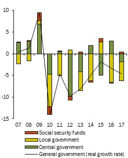 |
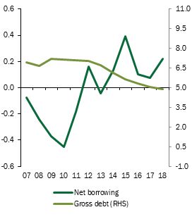 |
|
Source:
MEF analysis
based on ISTAT
and Bank of
Italy data.
|
|
___
13
Law No.
232/2016, Art.
1, para. 469.
14
Introduced by
Art. 28 of Law
No. 289/2002,
as governed by
Art. 14 of Law
No. 196/2009.
15
Provided by
Art. 13 of Law
No.196 of
2009.
16
Article 9,
paragraph 1-d,
Decree-Law No.
113/2016
(staff
recruitment
freeze) and
Art. 161,
para. 4,
Decree-Law No.
267/2000
(transfer
freeze for
local
authorities).
|
MINISTRY
OF ECONOMY AND
FINANCE
|
145
|
|
IV.
SENSITIVITY
AND
SUSTAINABILITY
OF PUBLIC
FINANCES
|
In
order to
promote
investment
across the
country, the
2019 Budget
Law17
strengthens
the investment
measures for
local
governments
launched in
2017-2018. The
first actions
focused on
financing the
final and
executive
planning of
municipalities
in Seismic
Hazard Zone 1
(extended to
Seismic Hazard
Zone 2 in
2018)18,
including 5
million for
2017, 25
million for
2018 and 30
million for
2019); next,
the 2018
Budget Law
provided for
investment
grants for
public works
to improve the
security of
buildings and
land, within
an overall
limit of 150
million for
2018, 300
million for
2019 and 400
million for
2020.
In
recognising
the sector and
the procedure
for
identifying
the
beneficiary
entities, the
2019 Budget
Law provides
for the
following
additional
medium-long
term financial
measures19:
| • |
contributions
to municipal
authorities
for small
works within
the overall
limit of 400
million for
2019 (Art. 1,
para. 107 to
114);
|
| • |
contributions
granted to
ordinary-statute
regions
towards for
public works
to improve the
safety of
buildings and
the local
area, within
the overall
limit of 135
million per
annum for the
period
2021-2025, 270
million for
2026, 315
million per
annum for the
period
2027-2032 and
360 million
for 2033 (Art.
1, para. 134
to 138);
|
| • |
contributions
granted to
municipalities
towards public
works to
improve the
safety of
buildings and
the local
area, in the
overall limit
of 250 million
per annum for
the period
2021-2025, 400
million for
2026, 450
million per
annum for the
period
2027-2031 and
500 million
for 2032 (Art.
1, para. 139
to 148);
|
| • |
contributions
towards the
construction
of healthcare
facilities,
within the
overall limit
of 100 million
per annum for
2021 and 2022,
300 million
per annum for
the period
2023-2025, 400
million per
annum for the
period
2026-2031, 300
million for
2032 and 200
million for
2033 (Art. 1,
para. 555 and
556);
|
| • |
contribution
granted to the
provincial
authorities of
ordinary-statute
regions for
roads and
schools, for a
total of 250
million per
annum for the
period
2019-2033
(Art. 1, c.
889 and 890);
|
| • |
investment
contributions
granted to
ordinary-statute
regions of 800
million for
2019, 908
million for
2020, 1,033
million per
annum for
2021-2022 and
468 million
for 2033
(Art.1, para.
833 et seq);
|
| • |
investment
contributions
granted under
the Agreements
with Special
Autonomous
Regions, for a
total of 2.486
million in the
period
2019-2033
(Art. 1, para.
126 and 875 et
seq.);
|
| • |
contributions
towards
improving
bridge safe,
for a total of
50 million per
annum for the
period
2019-2023
(Art. 1, para.
891);
|
| • |
contributions
granted to
Roma Capitale
towards the
extraordinary
restoration of
the surface of
major roads
and the
planning
review for the
completion of
Rome’s Metro
Line C, within
the overall
limit of 95
million for
2019, 85
million for
2020 and 20
million for
2021 (Art. 1,
para. 931 and
933).
|
___
17
Law No.
145/2018.
18
Laid down by
Article 41a of
Decree Law No.
50/2017.
19
Paragraphs 95
(Investment
fund of
central
administrations
of the State)
and 1028
(Hydrogeological
Risk) provide
resources
additional to
these
measures.
|
146
|
MINISTRY
OF ECONOMY AND
FINANCE
|
|
ECONOMIC
AND FINANCIAL
DOCUMENT -
SECT. I STABILITY
PROGRAMME
|
Health
Pact and
ceilings on
pharmaceutical
expenditure
Regional
healthcare
spending is
subject to the
rules
contained in
the Health
Pact, an
agreement with
a three-year
time horizon
between the
State, regions
and the
Autonomous
Provinces of
Trento and
Bolzano. Since
2000, these
agreements
have
established
the total
resources to
be allocated
to the
financing of
the National
Health Service
(SSN) in order
to ensure the
resources
needed for
medium-term
planning,
establishing
the sector’s
governance
tools and the
procedures to
monitor these
tools.
SSN
State funding
requires the
regions to
ensure balance
in the health
sector by
fully funding
any deficits.
Automatic
corrective
measures are
provided in
the event of
deviation from
balance, such
as increased
additional
regional
taxation on
individual
income and
IRAP and the
ban on retired
staff
turnover. An
essential tool
of governance
is the
requirement to
produce a
Recovery Plan
if the
regional
healthcare
sector has a
deficit
exceeding a
certain
threshold
established by
law or, even
if the deficit
is below the
aforesaid
threshold, if
the region has
no means of
funding or
presents
significant
deficiencies
in the quality
of care20.
The Plan
includes
measures to be
implemented to
restore a
balanced
budget over a
time horizon
of three years
and the
definition of
the
instruments
for monitoring
and verifying
its
implementation.
Lastly, the
legislation
requires
healthcare
sector to be
placed under
external
administration
if the
Recovery Plan
is
inadequately
prepared or
not
implemented
according to
the planned
schedule and
procedures. It
has recently
been
introduced
that whoever
holds the role
of
Commissioner
must not hold
any other
institutional
position in
the regional
authority
under
administration21.
Since 2016,
the submission
of Recovery
Plans is also
compulsory for
hospitals,
including
university
hospitals,
public care
and treatment
institutes and
other entities
that provide
care and
treatment
services,
should they
report
significant
imbalances
between
revenues and
costs22
or fail to
comply with
care quality
and
effectiveness
standards23.
The
latest Health
Pact was
stipulated on
10 July 2014
for the period
2014-2016. The
agreement
defined the
level of
financing
contributed by
the State and
dealt with
aspects of SSN
organisation
and
regulation.
The Pact was
transposed in
the Stability
Law for 2015.
For the years
following
2016, the most
recent
legislation
amendments
have redefined
the level of
SSN financing,
even in the
absence of a
new agreement.
Specifically,
the 2019
Budget Law
defines the
level of SSN
financing for
the three-year
period
2019-202124
at 114,474,
116,474 and
117,974
million,
respectively;
however,
access to the
increases
foreseen for
the years 2020
and 2021, as
compared to
2019, is
subject to the
conclusion of
a new Health
for the period
2019-2021. The
provisions
also identify
the main areas
of
intervention,
which should
be covered by
the Pact.
Dialogue
between
central
___
20
The 5 percent
threshold is
given by the
ratio between
the nominal
regional
deficit and
the total
resources
allocated by
the State to
finance the
regional
health
service.
21
Art. 25g of
Decree-Law No.
119/2018,
converted by
Law No.
136/2018.
22
Deviation
between costs
and revenues
greater than 7
percent of
revenues or
equal to at
least 7
million in
absolute
value.
23
Art. 1, para.
521-536, Law
No. 208/2015
(2016
Stability
Law).
24
Art. 1, para.
514, 518 and
526, Law No.
145/2018 (2019
Budget Law).
|
MINISTRY
OF ECONOMY AND
FINANCE
|
147
|
|
IV.
SENSITIVITY
AND
SUSTAINABILITY
OF PUBLIC
FINANCES
|
government
and regional
authorities
are currently
in progress to
reach
agreement on
the issues.
Since
2017, part of
the standard
national
health
financing
requirement,
equal to 1
billion, has
been earmarked
for the
purchase of
particular
types of
drugs, of
which 500
million for
innovative
drugs and 500
million for
cancer drugs.
The
ceilings on
pharmaceutical
spending,
substantially
modified by
the 2017
Budget Law,
are confirmed.
Specifically,
the existing
ceilings are
set at 7.96
percent of SSN
financing for
pharmaceutical
spending under
the national
healthcare
system25
and 6.89
percent for
direct
purchases26.
The
automatic
correction
mechanism
(payback)
remains in
force in case
of ceilings
overrun. In
the event of
overrun of the
ceiling of
pharmaceutical
spending under
the national
healthcare
system, the
excess must be
funded by the
chain of
pharmaceutical
operators
(producers,
wholesalers,
pharmacies);
for overruns
of ceiling on
pharmaceutical
spending for
direct
purchases, 50
percent of the
excess is
charged to the
regional
authorities
and the
remaining 50
percent to the
pharmaceutical
companies.
With effect
from 2019, the
2019 Budget
Law introduced
simplified
procedures to
determine the
pharmaceutical
spending
payback for
direct
purchases,
which require
inter alia
that the
Italian Drug
Agency (AIFA)
use data from
electronic
invoices to
monitor
expenditure.
This should
make basic
information
more reliable
and should
therefore
prevent, or at
least limit,
the ongoing
litigation
that the
pharmaceutical
companies
began in 2013.
The final
settlement of
the
aforementioned
litigation
should instead
be ensured by
the provisions
introduced by
Decree-Law No.
135/2018,
converted by
Law No.
12/201927,
which
establish
that, in the
event that the
pharmaceutical
companies pay
into the State
budget a total
of 2,378
million by 30
April 2019,
including sums
already paid
for the period
2013-2017, the
litigation
concerning the
above-mentioned
annuities
shall be
understood to
be expired due
to termination
of cause for
litigation.
___
25
Pharmaceutical
spending under
the national
healthcare
system refers
to spending on
refundable
medicines,
excluding
patient
contributions,
distributed
through
affiliated
public and
private
pharmacies.
26
Pharmaceutical
spending for
direct
purchases
refers to
spending on
drugs
purchased
directly by
healthcare
companies,
distributed in
hospitals or
distributed
directly by
these
companies in
the local
area. This
distribution
can also be
undertaken
through
specific
agreements
with
affiliated
pharmacies.
The one
billion share
of spending
set aside for
innovative and
cancer drugs
from 2017 is
excluded from
ceiling
calculations.
27
Art. 9a, para.
3-6.
|
148
|
MINISTRY
OF ECONOMY AND
FINANCE
|
The
ECONOMIC
AND FINANCIAL
DOCUMENT 2019
is
available
on-line
at the
internet
address listed
below:
www.mef.gov.it • www.dt.tesoro.it • www.rgs.mef.gov.it
ISSN
2239-5539